Performance Analysis Recap Concurrency, Parallelism, Distributed computing Two parallelization approaches for summation computation Comparing two Attempts Parallel computation (1) Compute partial sum of np elements. Serial computation (2)
"Performance Analysis Recap Concurrency," is the property of its rightful owner. Permission is granted to
download and print the materials on this website for personal, non-commercial use only, and to display it
on your personal computer provided you do not modify the materials and that you retain all copyright
notices contained in the materials. By downloading content from our website, you accept the terms of this
agreement.
Two parallelization approaches for summation computation<br>
03
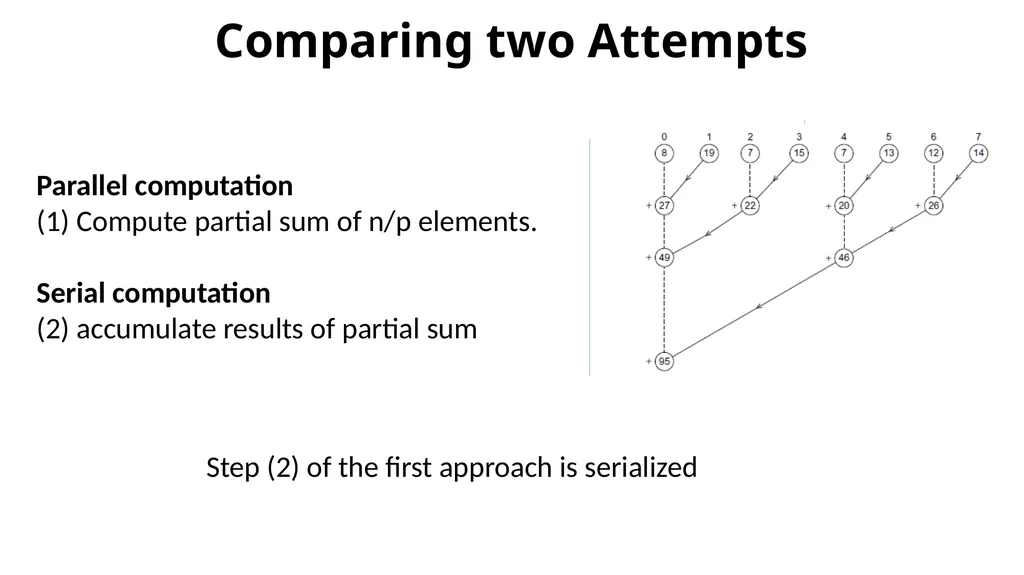
Comparing two Attempts Parallel computation
(1) Compute partial sum of n/p elements.
Serial computation
(2) accumulate results of partial sum Step (2) of the first approach is serialized<br>
04
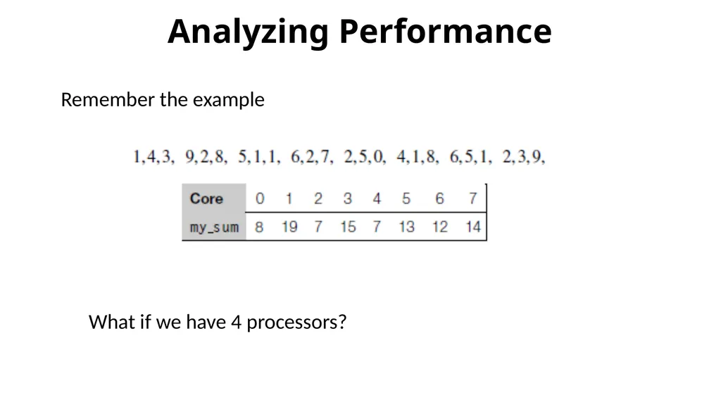
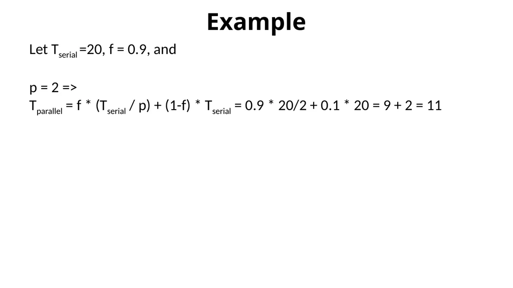
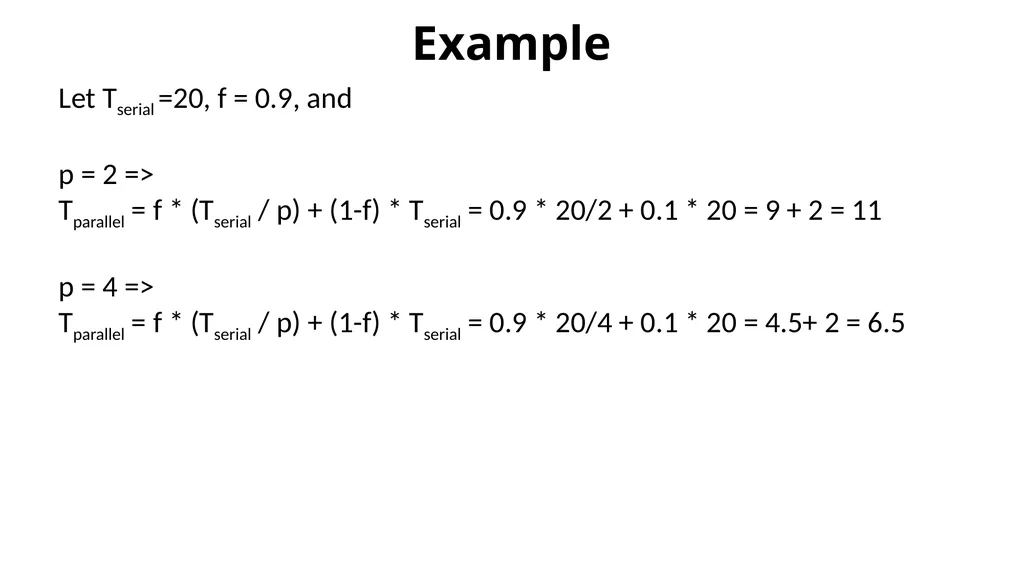
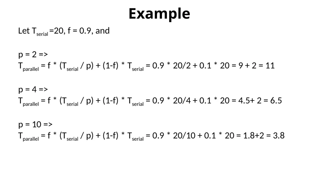
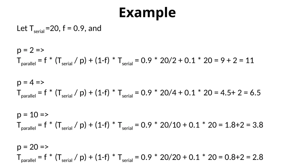
Analyzing Performance Remember the example What if we have 4 processors?<br>
05
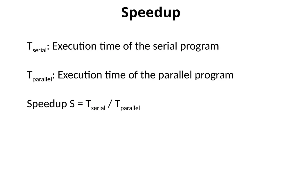
Speedup Tserial: Execution time of the serial program
Tparallel: Execution time of the parallel program
Speedup S = Tserial / Tparallel<br>
06
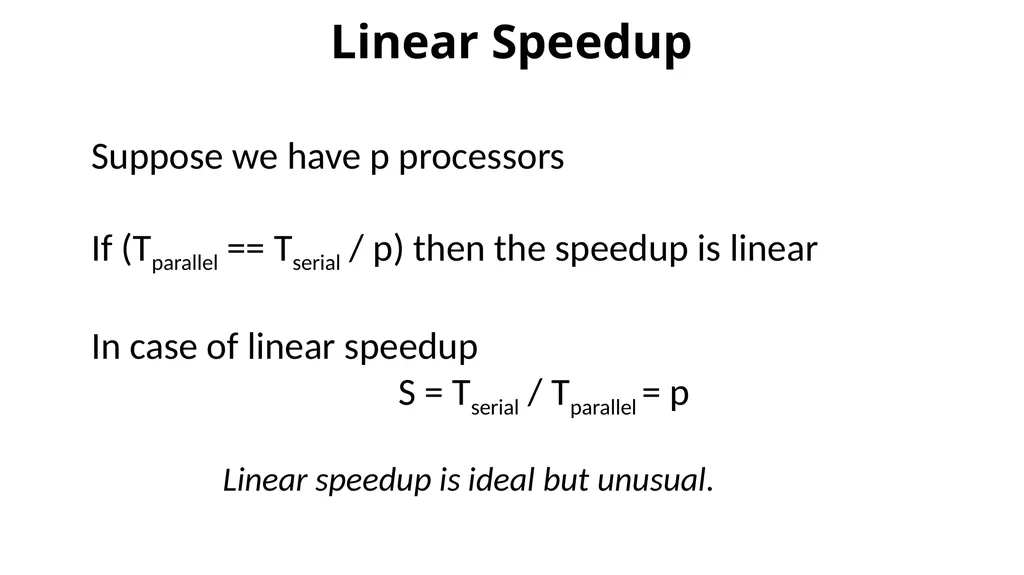
Linear Speedup Suppose we have p processors
If (Tparallel == Tserial / p) then the speedup is linear
In case of linear speedup
S = Tserial / Tparallel = p Linear speedup is ideal but unusual.<br>
07
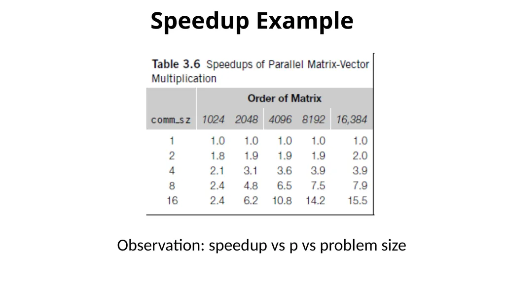
Speedup Example Observation: speedup vs p vs problem size<br>
08
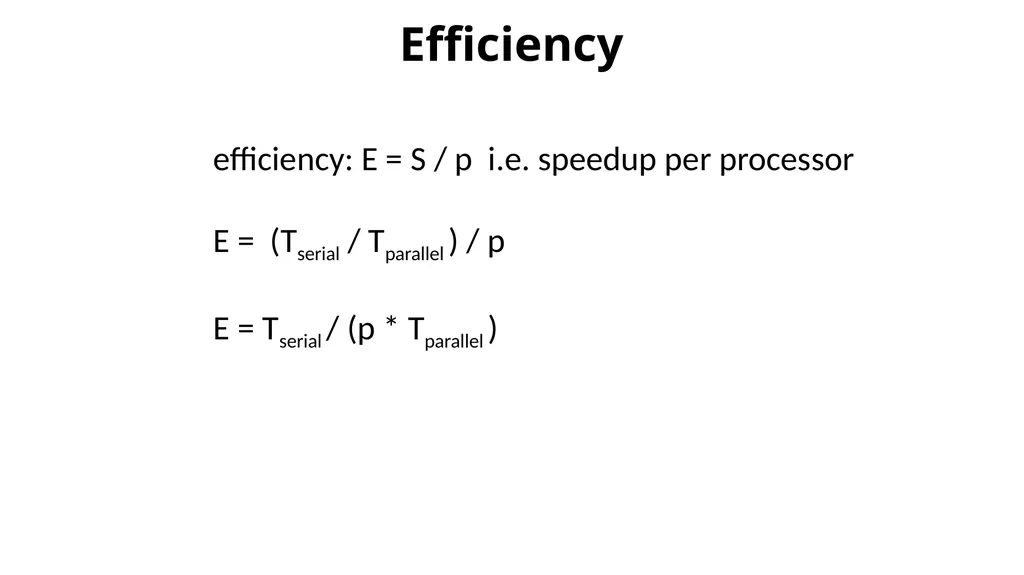
Efficiency efficiency: E = S / p i.e. speedup per processor
E = (Tserial / Tparallel ) / p
E = Tserial / (p * Tparallel )<br>
09
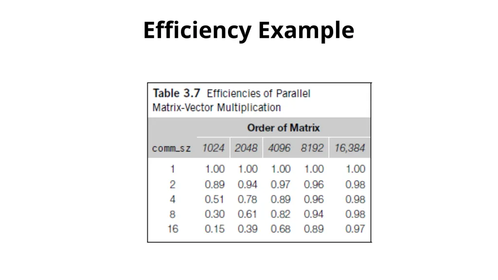
Efficiency Example<br>
10
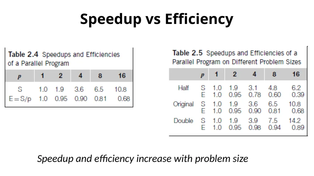
Speedup vs Efficiency Speedup and efficiency increase with problem size<br>
11
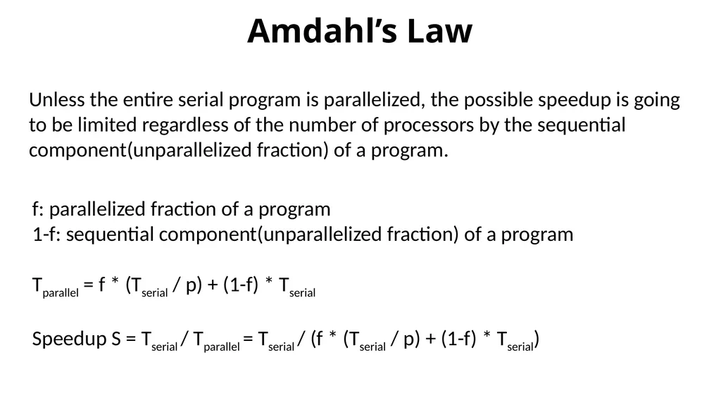
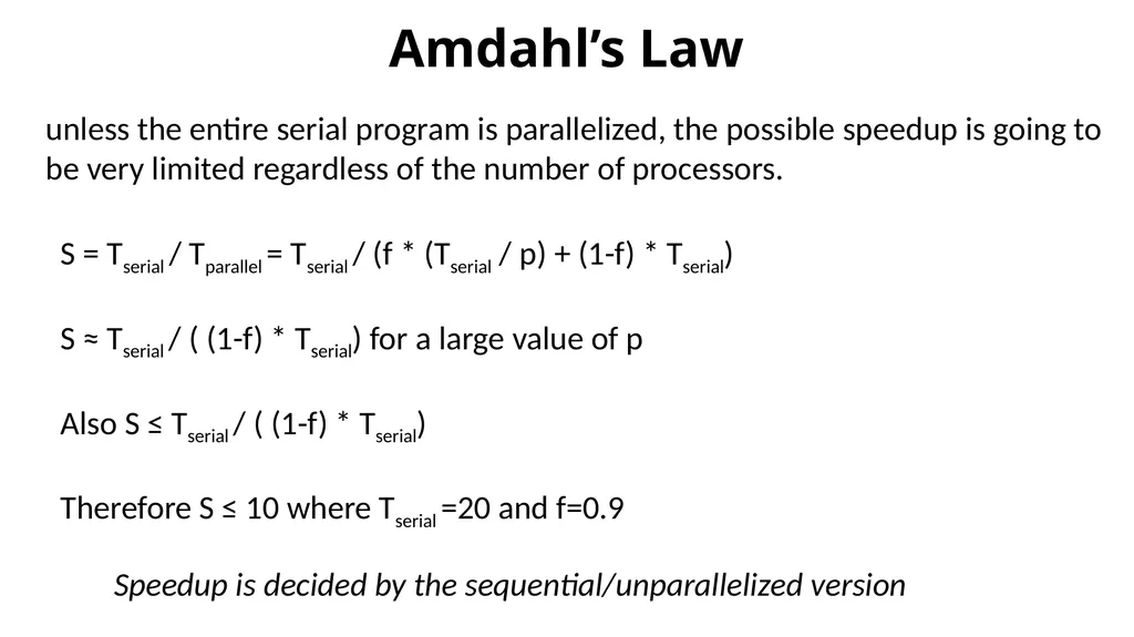
Amdahl’s Law Unless the entire serial program is parallelized, the possible speedup is going to be limited regardless of the number of processors by the sequential component(unparallelized fraction) of a program. f: parallelized fraction of a program
1-f: sequential component(unparallelized fraction) of a program
Amdahl’s Law unless the entire serial program is parallelized, the possible speedup is going to be very limited regardless of the number of processors. S = Tserial / Tparallel = Tserial / (f * (Tserial / p) + (1-f) * Tserial)
S ≈ Tserial / ( (1-f) * Tserial) for a large value of p
Also S ≤ Tserial / ( (1-f) * Tserial)
Therefore S ≤ 10 where Tserial =20 and f=0.9 Speedup is decided by the sequential/unparallelized version<br>
17
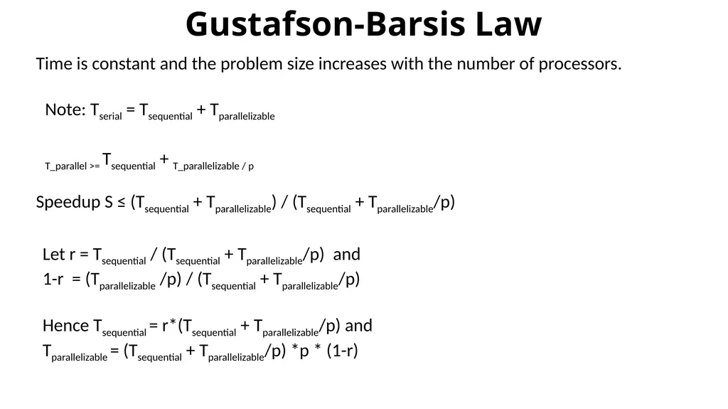
Gustafson-Barsis Law Time is constant and the problem size increases with the number of processors. Speedup S ≤ (Tsequential + Tparallelizable) / (Tsequential + Tparallelizable/p) Note: Tserial = Tsequential + Tparallelizable
T_parallel >= Tsequential + T_parallelizable / p Let r = Tsequential / (Tsequential + Tparallelizable/p) and
1-r = (Tparallelizable /p) / (Tsequential + Tparallelizable/p)
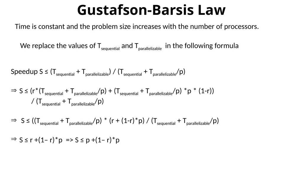
Gustafson-Barsis Law Time is constant and the problem size increases with the number of processors. Speedup S ≤ (Tsequential + Tparallelizable) / (Tsequential + Tparallelizable/p)
S ≤ r +(1– r)*p => S ≤ p +(1– r)*p We replace the values of Tsequential and Tparallelizable in the following formula<br>
19
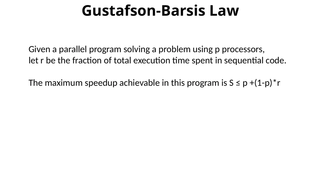
Gustafson-Barsis Law Given a parallel program solving a problem using p processors,
let r be the fraction of total execution time spent in sequential code.
The maximum speedup achievable in this program is S ≤ p +(1-p)*r<br>
20
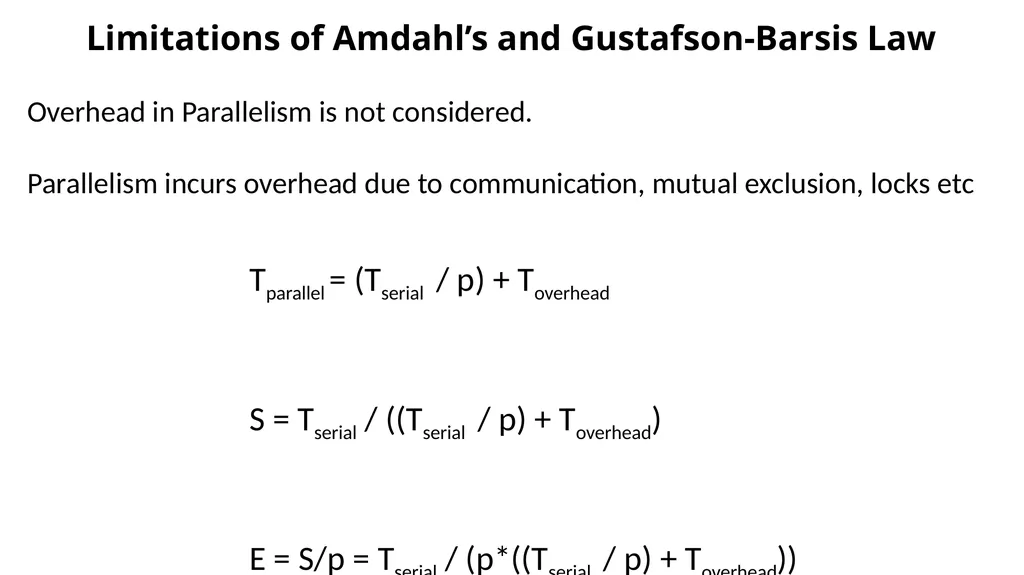
Limitations of Amdahl’s and Gustafson-Barsis Law Overhead in Parallelism is not considered.
Parallelism incurs overhead due to communication, mutual exclusion, locks etc Tparallel = (Tserial / p) + Toverhead