Principal components analysis Gavin Band Why do PCA? PCA is good at detecting directions of major variation in your data. This might be: Population structure subpopulations having different allele frequencies. Unexpected (cryptic)
"Principal components analysis Gavin Band Why do" is the property of its rightful owner. Permission is granted to
download and print the materials on this website for personal, non-commercial use only, and to display it
on your personal computer provided you do not modify the materials and that you retain all copyright
notices contained in the materials. By downloading content from our website, you accept the terms of this
agreement.
Presentation Transcript
01
Principal components analysis Gavin Band<br>
02
Why do PCA? PCA is good at detecting “directions” of major variation in your data. This might be:
Population structure – subpopulations having different allele frequencies.
Unexpected (“cryptic”) relationships.
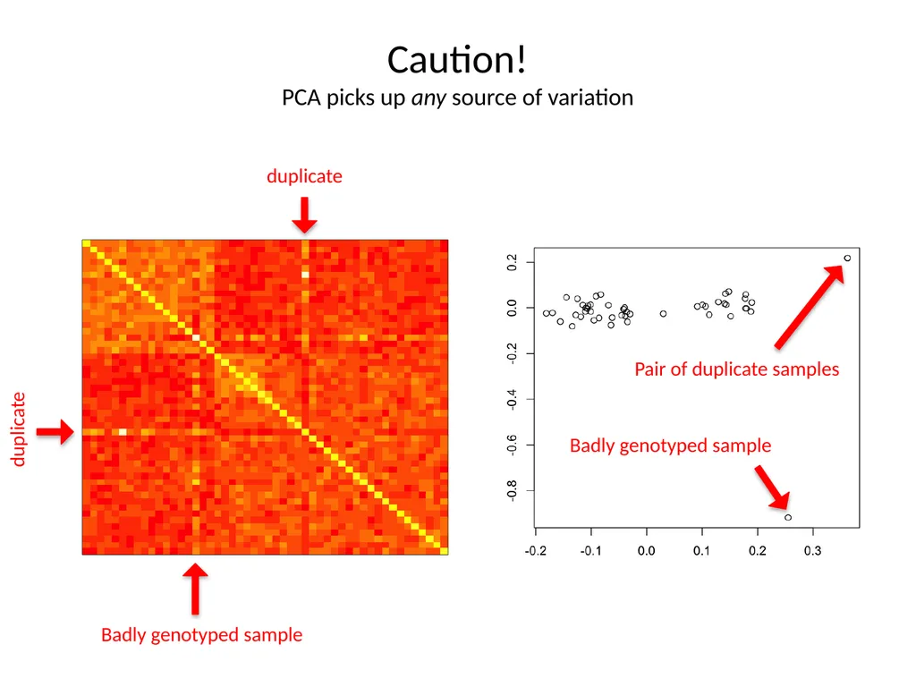
Artifacts such as genotyping errors, etc.
Apart from intrinsic interest, these are precisely the factors that need to be controlled for in association tests.<br>
03
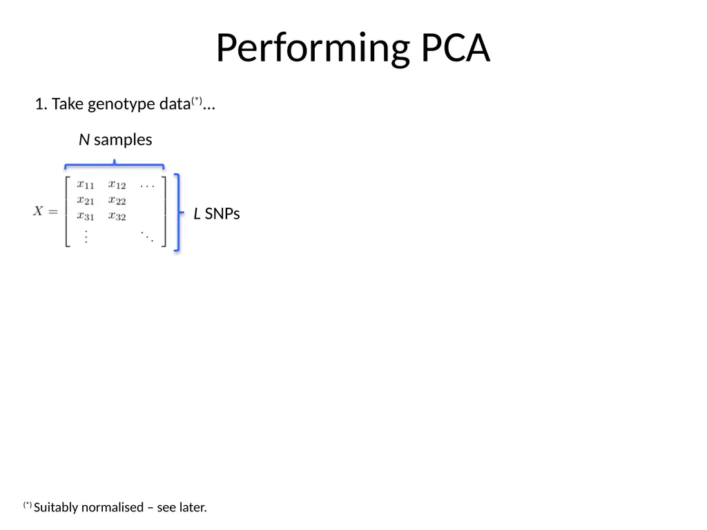
Performing PCA L SNPs N samples 1. Take genotype data(*)... (*) Suitably normalised – see later.<br>
04
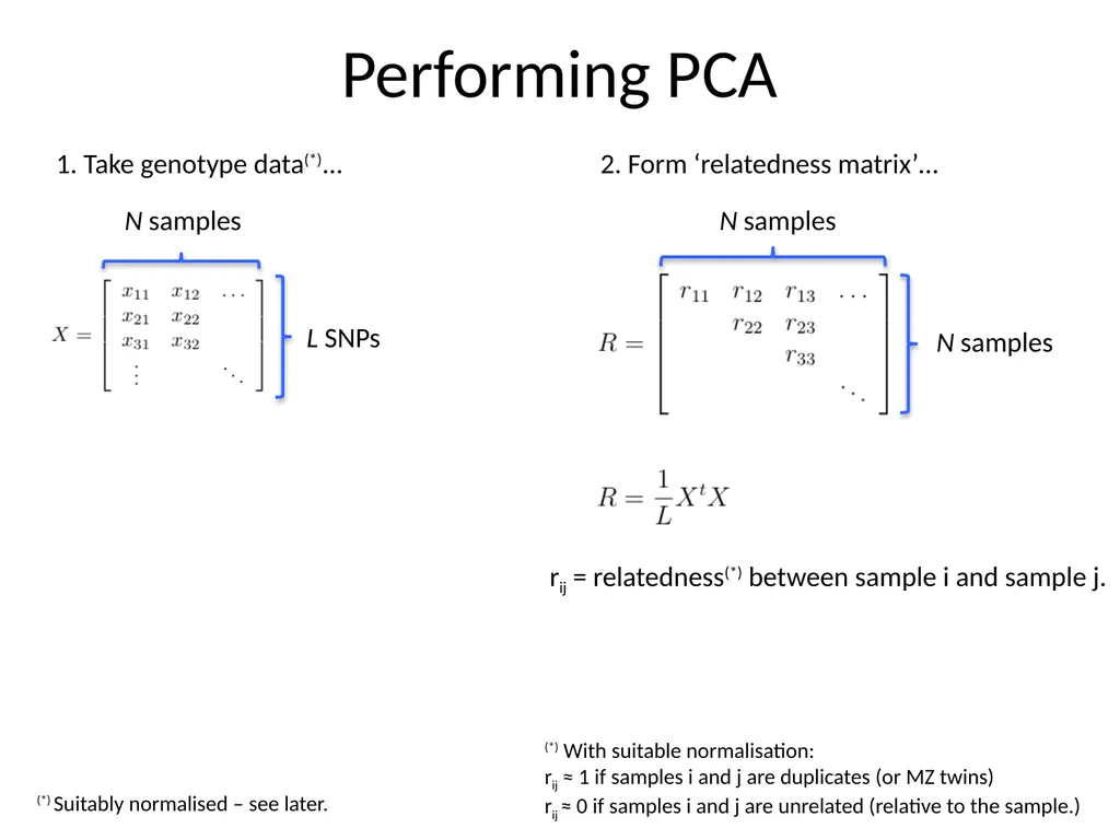
Performing PCA L SNPs N samples 1. Take genotype data(*)... 2. Form ‘relatedness matrix’… N samples (*) With suitable normalisation:
rij ≈ 1 if samples i and j are duplicates (or MZ twins)
rij ≈ 0 if samples i and j are unrelated (relative to the sample.) rij = relatedness(*) between sample i and sample j. (*) Suitably normalised – see later. N samples<br>
05
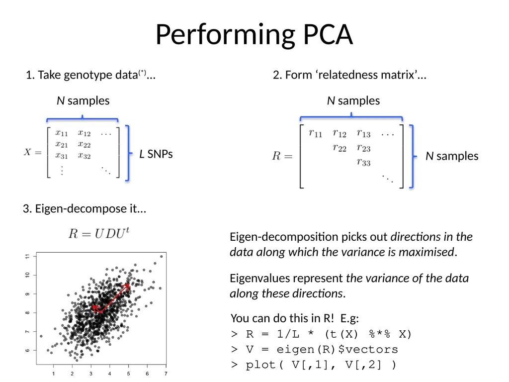
Performing PCA L SNPs N samples 1. Take genotype data(*)... 3. Eigen-decompose it... Eigen-decomposition picks out directions in the data along which the variance is maximised. You can do this in R! E.g:
> R = 1/L * (t(X) %*% X)
> V = eigen(R)$vectors
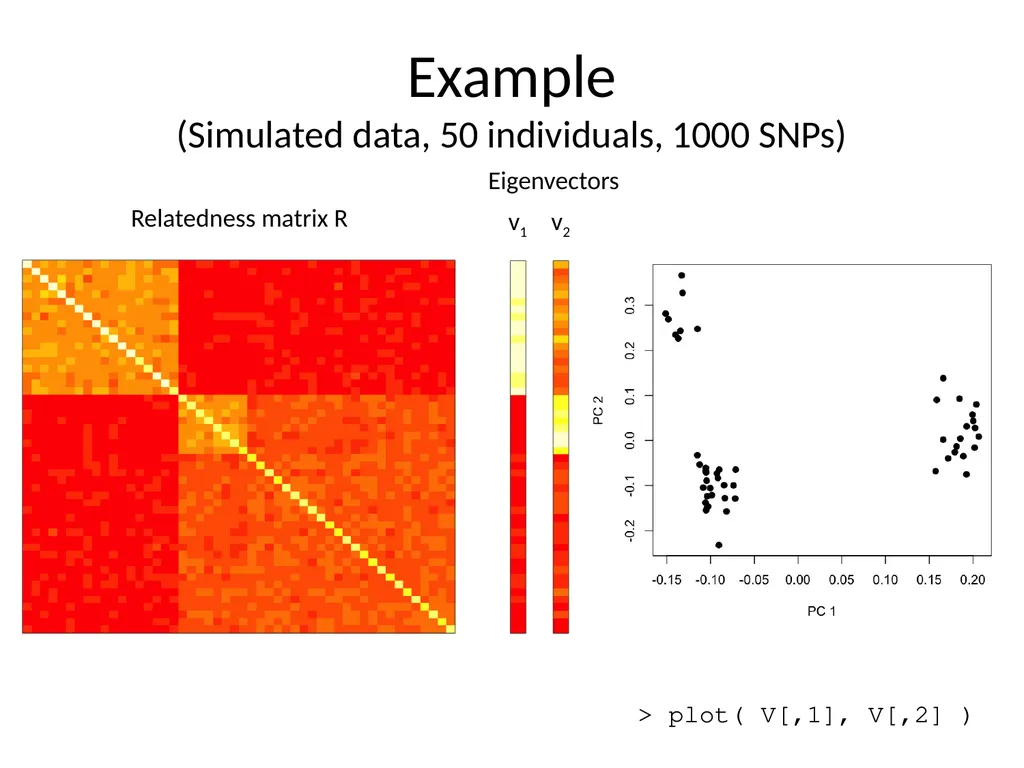
> plot( V[,1], V[,2] ) 2. Form ‘relatedness matrix’… N samples N samples Eigenvalues represent the variance of the data along these directions.<br>
06
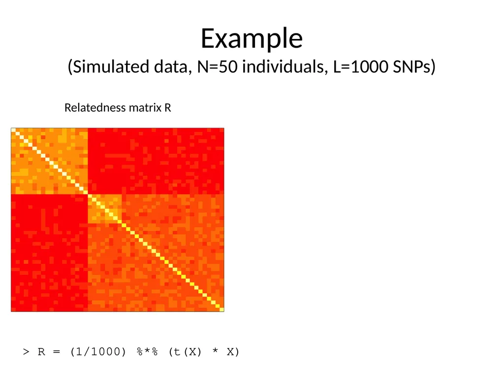
Example (Simulated data, N=50 individuals, L=1000 SNPs) Relatedness matrix R > R = (1/1000) %*% (t(X) * X)<br>
07
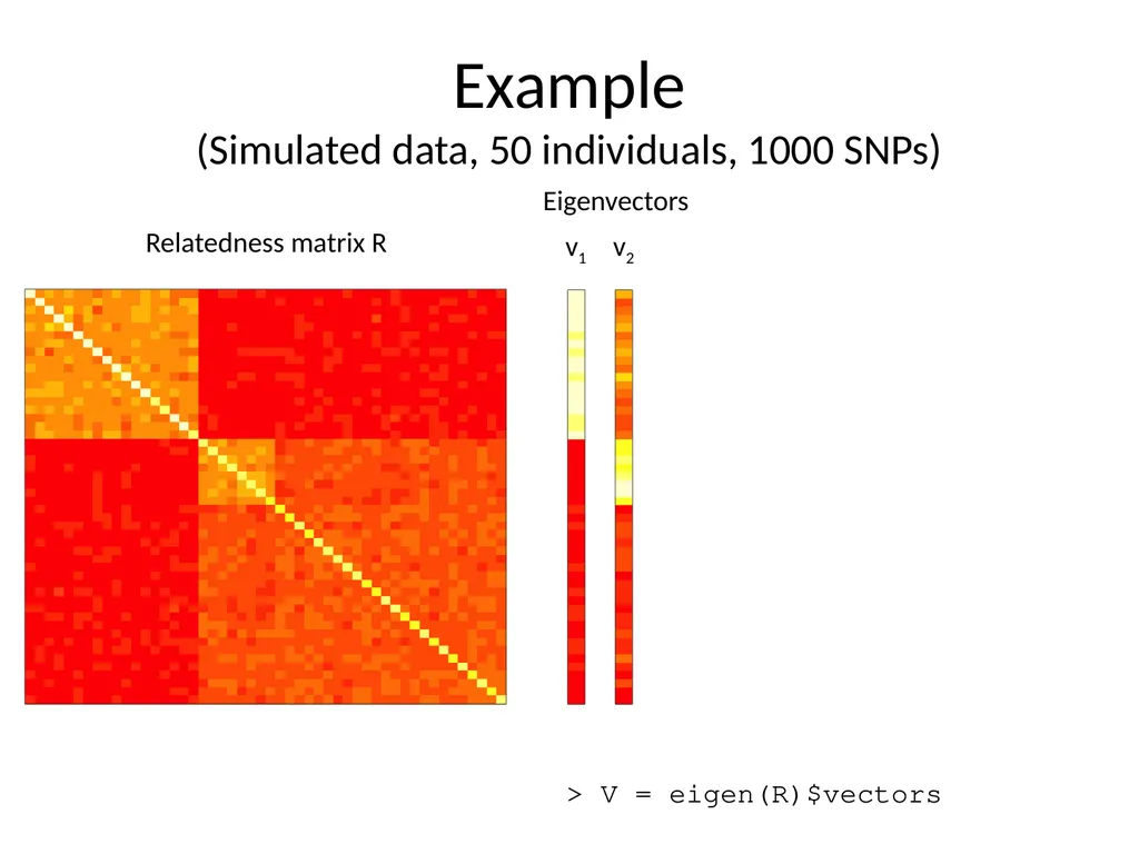
Example (Simulated data, 50 individuals, 1000 SNPs) Relatedness matrix R Eigenvectors v1 v2 > V = eigen(R)$vectors<br>
08
Example (Simulated data, 50 individuals, 1000 SNPs) Relatedness matrix R v1 v2 Eigenvectors > plot( V[,1], V[,2] )<br>
09
Caution! PCA picks up any source of variation Pair of duplicate samples Badly genotyped sample duplicate duplicate Badly genotyped sample<br>
10
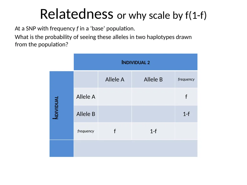
Relatedness or why scale by f(1-f) At a SNP with frequency f in a ‘base’ population.
What is the probability of seeing these alleles in two haplotypes drawn from the population?<br>
11
“Unrelated” individuals
Alleles drawn independently At a SNP with frequency f in a ‘base’ population.
What is the probability of seeing these alleles in two haplotypes drawn from the population? Relatedness or why scale by f(1-f)<br>
12
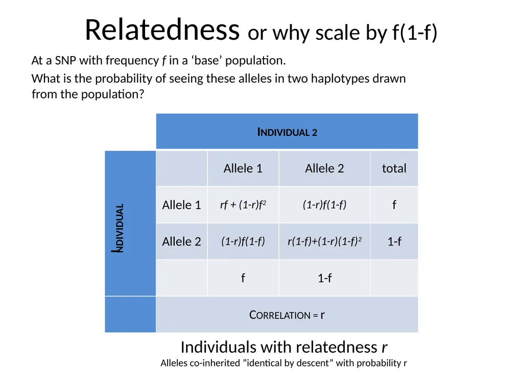
Relatedness or why scale by f(1-f) At a SNP with frequency f in a ‘base’ population.
What is the probability of seeing these alleles in two haplotypes drawn from the population? Individuals with relatedness r
Alleles co-inherited ”identical by descent” with probability r<br>
13
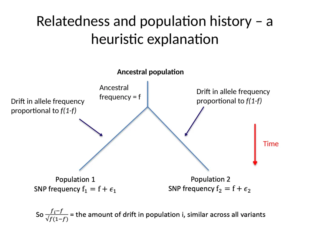
Relatedness and population history – a heuristic explanation Drift in allele frequency proportional to f(1-f) Drift in allele frequency proportional to f(1-f) Ancestral population Ancestral frequency = f Time<br>
14
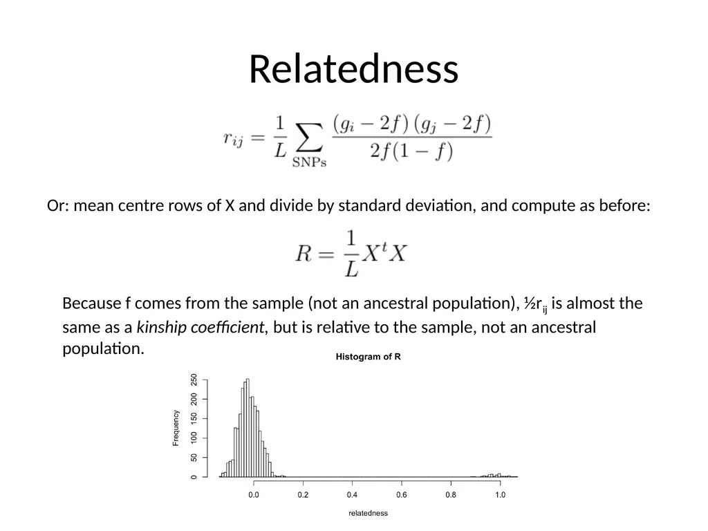
Relatedness Or: mean centre rows of X and divide by standard deviation, and compute as before: Because f comes from the sample (not an ancestral population), ½rij is almost the same as a kinship coefficient, but is relative to the sample, not an ancestral population.<br>
15
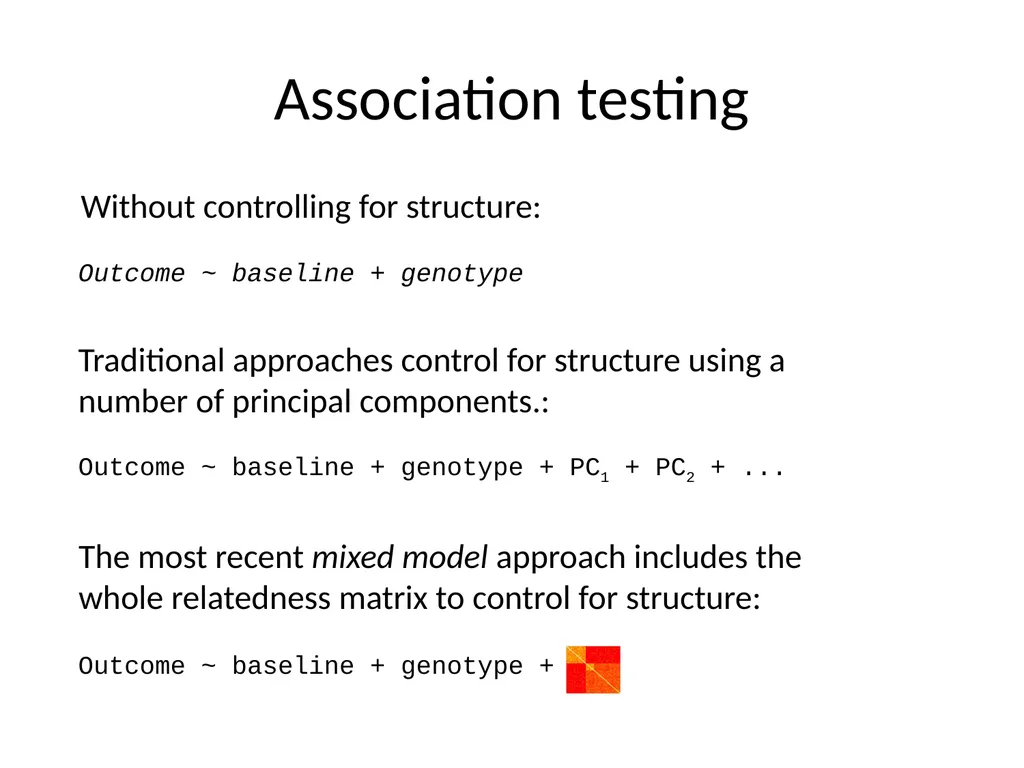
Association testing Outcome ~ baseline + genotype Outcome ~ baseline + genotype + PC1 + PC2 + ... Outcome ~ baseline + genotype + Without controlling for structure: Traditional approaches control for structure using a number of principal components.: The most recent mixed model approach includes the whole relatedness matrix to control for structure:<br>
16
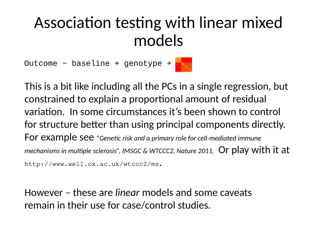
Association testing with linear mixed models Outcome ~ baseline + genotype + This is a bit like including all the PCs in a single regression, but constrained to explain a proportional amount of residual variation. In some circumstances it’s been shown to control for structure better than using principal components directly. For example see “Genetic risk and a primary role for cell-mediated immune mechanisms in multiple sclerosis”, IMSGC & WTCCC2, Nature 2011. Or play with it at http://www.well.ox.ac.uk/wtccc2/ms. However – these are linear models and some caveats remain in their use for case/control studies.<br>
17
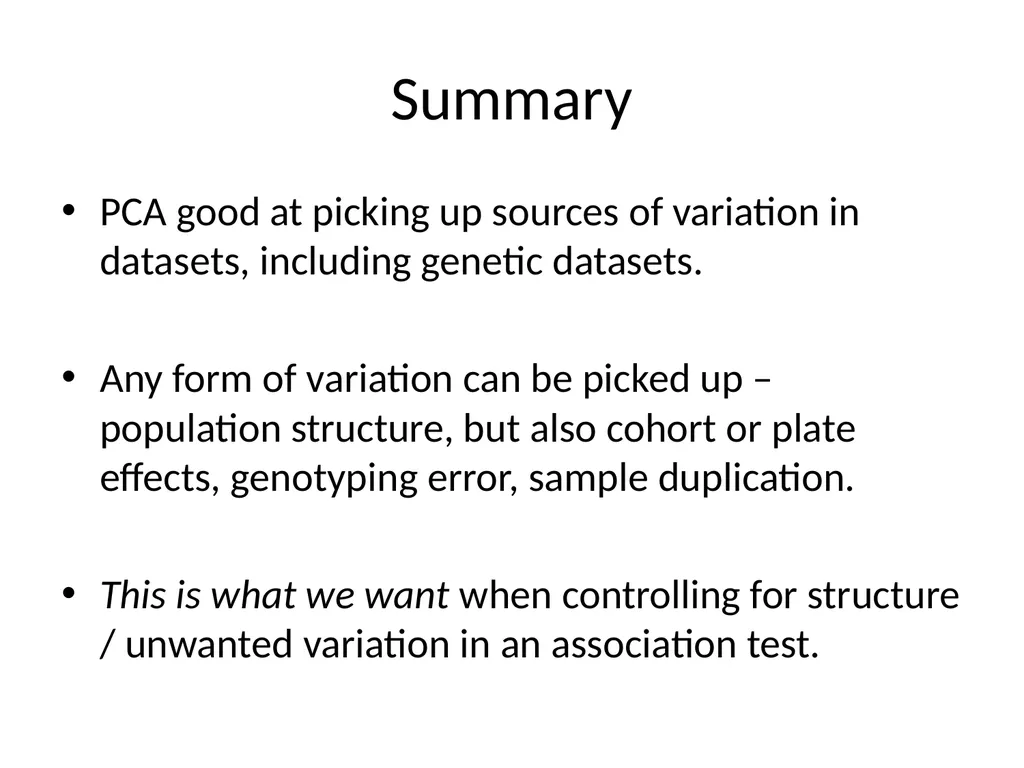
Summary PCA good at picking up sources of variation in datasets, including genetic datasets.
Any form of variation can be picked up – population structure, but also cohort or plate effects, genotyping error, sample duplication.
This is what we want when controlling for structure / unwanted variation in an association test.<br>
18
Software for performing PCA Plink (v1.9 or above)
http://www.cog-genomics.org/plink2