
Purely sequence-trained neural networks for ASR


Description: Purely sequence-trained neural networks for ASR based on lattice-free MMI Dan Povey, Vijay Peddinti, Daniel Galvez, Pegah Ghahremani, Vimal Manohar, Xingyu Na, Yiming Wang, Sanjeev Khudanpur Why should you care about this ? It gives better
Related Topics
Download Presentation
"Purely sequence-trained neural networks for ASR" is the property of its rightful owner. Permission is granted to download and print the materials on this website for personal, non-commercial use only, and to display it on your personal computer provided you do not modify the materials and that you retain all copyright notices contained in the materials. By downloading content from our website, you accept the terms of this agreement.
Presentation Transcript
slide1. Purely sequence-trained neural networks for ASR based on lattice-free MMI Dan Povey, Vijay Peddinti, Daniel Galvez, Pegah Ghahremani, Vimal Manohar, Xingyu Na, Yiming Wang, Sanjeev Khudanpur<br>
slide2. Why should you care about this ? It gives better WERs than the conventional way of training models.
It's a lot faster to train
It's a lot faster to decode
We're modifying most of the recipes in Kaldi to use this.
Doesn't always give WER improvements on small data (e.g. < 50 hours)<br>
slide3. Connection with CTC This actually came out from some (unpublished) work on CTC.
It's a simplification of an extension of an extension of CTC.
Not really going into that work in the paper or talk. Basically I didn't see any gains with any variety of CTC (many others find this too).
Commonalities with CTC:
Objective function is posterior of the correct transcript of the utterance
30ms frame shift at the output
(see at this conf., "Lower Frame Rate NN AMs", Pundak & Sainath)<br>
slide4. What is it ? It's MMI, captain, but not as we know it.
Normally we'd do frame-by-frame training followed by MMI.
We train the neural net from a random start.
The frame shift [at the neural net output] is 30ms, not 10ms.<br>
slide5. Why is training MMI from scratch hard? In MMI training, in general there are two forward-backward algorithms, and we subtract the occupation counts (num-den)
Numerator == correct transcript
Denominator == all possible transcripts
Full forward backward or even search over denominator is slow -> must be on GPU.
On GPU, beam search is hard
Lose a lot of efficiency if different cores are taking different code paths or accessing different data<br>
slide6. How do we do it? Full forward backward of denominator
(on GPU, custom kernels)
Break up utterances into fixed-size chunks
(one-second chunks)
Keep the denominator graph small enough
so we can keep the forward (𝛼) scores on the GPU for a minibatch of utterances (e.g. 128).
In next slides, will explore the consequences of these decisions.<br>
slide7. Fixed chunk sizes Use 1-second chunks
(not highly sensitive to the exact length)
Slight overlaps or gaps where we break up utterances this way
Append successive utterances in data preparation
so all utterances are at least 1 second.
Difficulty: how do we break up the transcripts?
1-second chunks may not coincide with word boundaries.
... see next slide for solution.<br>
slide8. Numerator representation Generate a lattice for the numerator, encoding alternative pronunciations of the transcript of the original utterance.
The lattice is turned into an FST that constrains at what time the phones can appear, to +-0.05 seconds from their positions in the lattice1.
Process this into an FST whose labels are pdfs (neural-net outputs).
Extract fixed-size chunks from this FST 1. In [1], FSTs are used to constrain the labels to a certain window around where the baseline system puts them. We used the same idea here.
[1] : A. Senior, H. Sak, F. de Chaumont Quitry, T. N. Sainath, and K. Rao, “Acoustic Modelling with CD-CTC-SMBR LSTM RNNS,” in ASRU, 2015.<br>
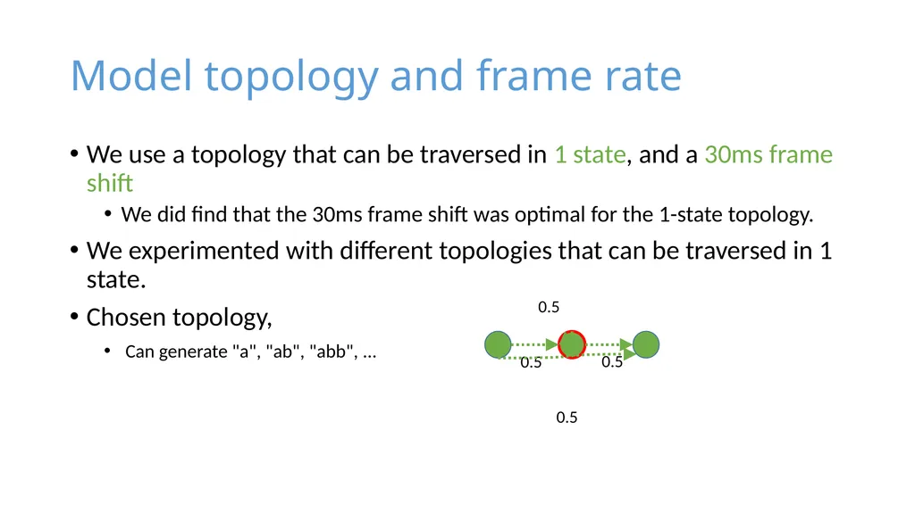
slide9. Model topology and frame rate We use a topology that can be traversed in 1 state, and a 30ms frame shift
We did find that the 30ms frame shift was optimal for the 1-state topology.
We experimented with different topologies that can be traversed in 1 state.
Chosen topology,
Can generate "a", "ab", "abb", ...<br>
slide10. Denominator graph Denominator graph is like a decoding graph FST (HCLG).
Phone-level language model and no lexicon
so it's like HCP, where P is the phone LM.
We construct P to minimize the size of HCP.
It's a 4-gram, but with no backoff lower than 3-gram
(so that triphones not seen in training cannot be generated).
The number of states is limited by completely removing low-count 4-gram states
(backing off the counts to 3-gram).
We minimize the size of the final graph
a different-than-normal graph construction recipe<br>
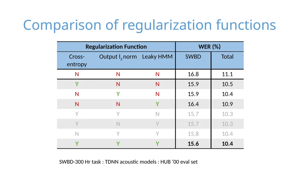
slide11. Regularization Very vulnerable to over-training
Three regularization methods:
L2 regularization on the network output*
Cross-entropy regularization
Add a separate cross-entropy layer that's trained but is then thrown away (that shares the hidden layers).
"Leaky HMM".
This refers to modifying the denominator-graph so that it is "stopped and restarted" with a small probability (e.g. 0.1) on each frame [like forgetting the context].
The gains from these regularization methods are somewhat additive; we use all three (and also use smaller-than-normal models). * the outputs are in log space, they are like pseudo-likelihoods.<br>
slide12. Frame shift issues In our neural nets, the input frame shift is 10ms and the output frame shift is 30ms.
This is not quite equivalent to splicing the input, because the early TDNN and LSTM layers use frame offsets and recurrence delays that are not multiples of 30ms.
We try to keep all such frame offsets in later layers of the network as multiples of 3 so that those layers only need to be evaluated every 3 frames.
The neural network is obviously about 3 times faster to evaluate than for regular models (perhaps more, since model is smaller).
In training, on each epoch we cycle through 3 differently-shifted versions of the training data (shifted by -1, 0, 1 input frame).<br>
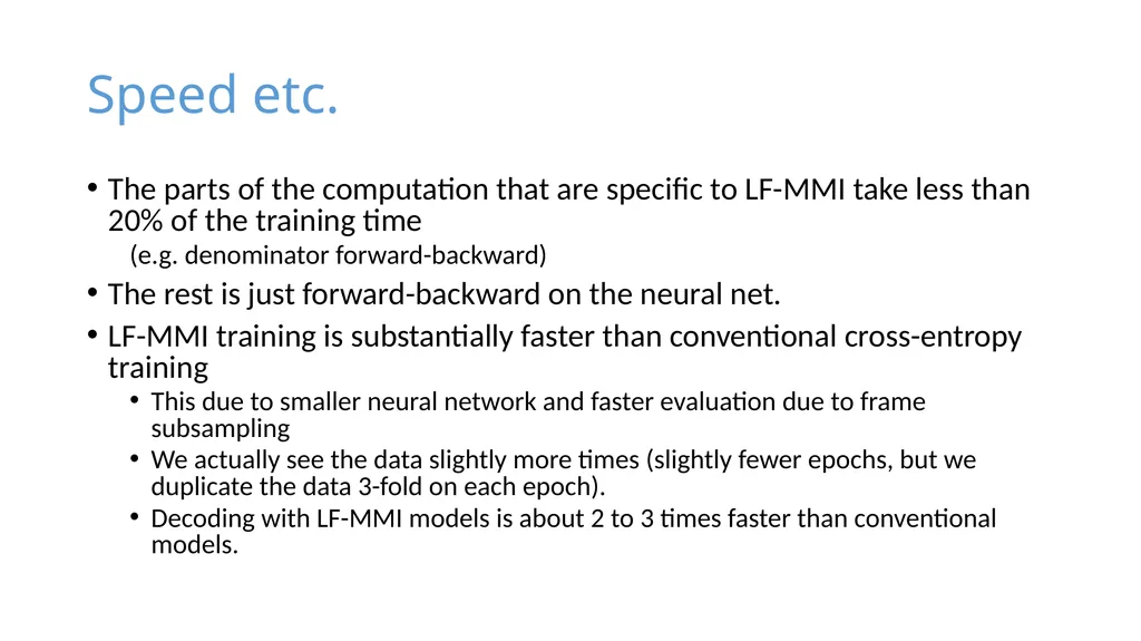
slide13. Speed etc. The parts of the computation that are specific to LF-MMI take less than 20% of the training time
(e.g. denominator forward-backward)
The rest is just forward-backward on the neural net.
LF-MMI training is substantially faster than conventional cross-entropy training
This due to smaller neural network and faster evaluation due to frame subsampling
We actually see the data slightly more times (slightly fewer epochs, but we duplicate the data 3-fold on each epoch).
Decoding with LF-MMI models is about 2 to 3 times faster than conventional models.<br>
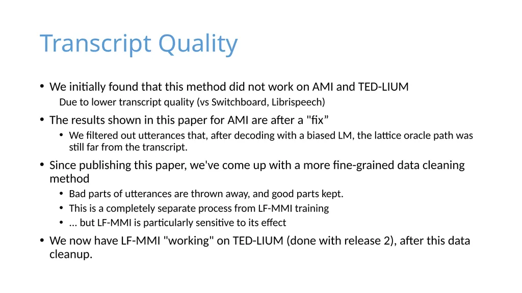
slide14. Transcript Quality We initially found that this method did not work on AMI and TED-LIUM
Due to lower transcript quality (vs Switchboard, Librispeech)
The results shown in this paper for AMI are after a "fix”
We filtered out utterances that, after decoding with a biased LM, the lattice oracle path was still far from the transcript.
Since publishing this paper, we've come up with a more fine-grained data cleaning method
Bad parts of utterances are thrown away, and good parts kept.
This is a completely separate process from LF-MMI training
... but LF-MMI is particularly sensitive to its effect
We now have LF-MMI "working" on TED-LIUM (done with release 2), after this data cleanup.<br>
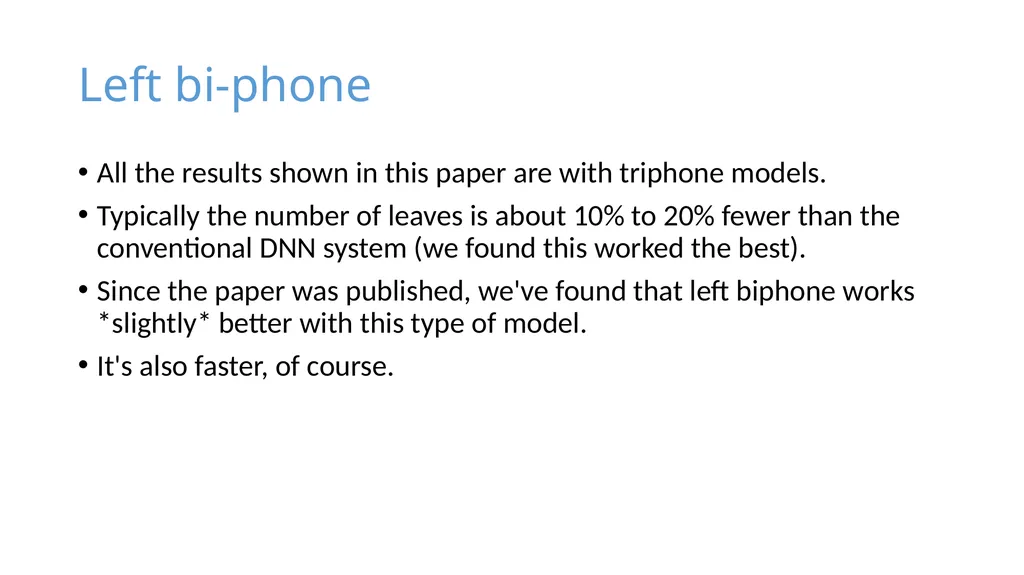
slide15. Left bi-phone All the results shown in this paper are with triphone models.
Typically the number of leaves is about 10% to 20% fewer than the conventional DNN system (we found this worked the best).
Since the paper was published, we've found that left biphone works *slightly* better with this type of model.
It's also faster, of course.<br>
slide16. Results<br>
slide17. Comparison of regularization functions SWBD-300 Hr task : TDNN acoustic models : HUB ‘00 eval set<br>
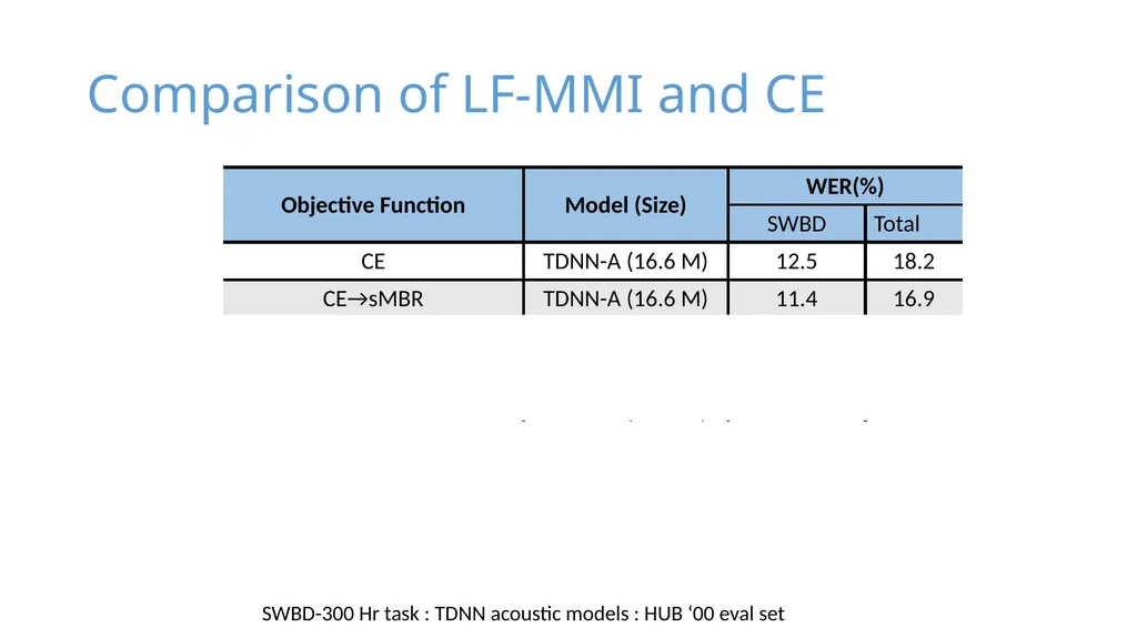
slide18. Comparison of LF-MMI and CE SWBD-300 Hr task : TDNN acoustic models : HUB ‘00 eval set<br>
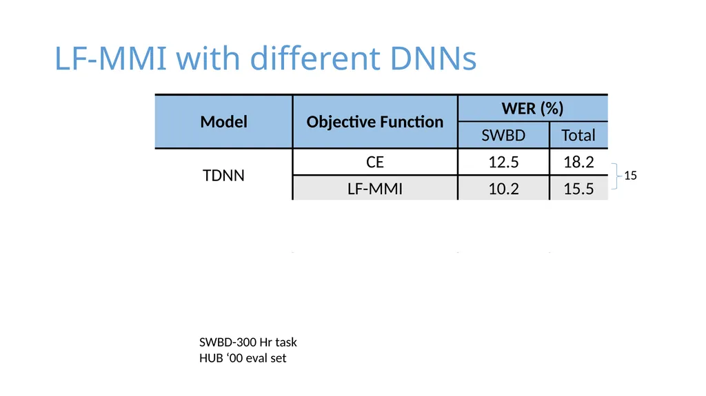
slide19. LF-MMI with different DNNs 15 SWBD-300 Hr task
HUB ‘00 eval set<br>
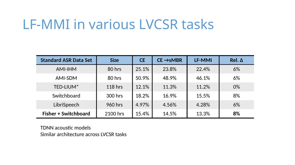
slide20. LF-MMI in various LVCSR tasks TDNN acoustic models
Similar architecture across LVCSR tasks<br>
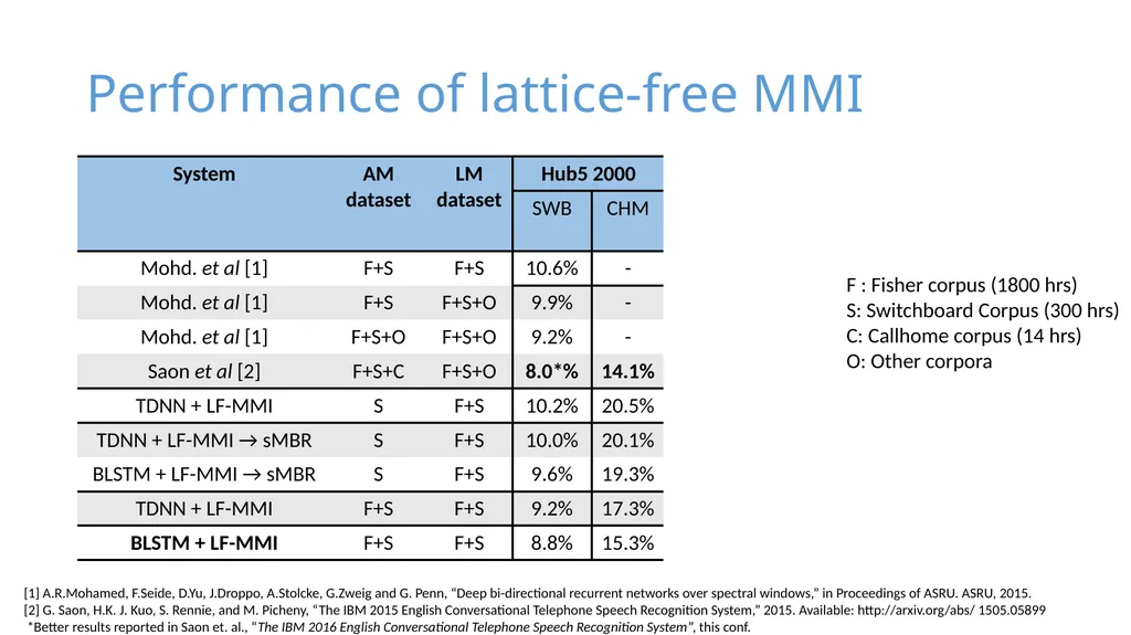
slide21. Performance of lattice-free MMI F : Fisher corpus (1800 hrs)
S: Switchboard Corpus (300 hrs)
C: Callhome corpus (14 hrs)
O: Other corpora [1] A.R.Mohamed, F.Seide, D.Yu, J.Droppo, A.Stolcke, G.Zweig and G. Penn, “Deep bi-directional recurrent networks over spectral windows,” in Proceedings of ASRU. ASRU, 2015.
[2] G. Saon, H.K. J. Kuo, S. Rennie, and M. Picheny, “The IBM 2015 English Conversational Telephone Speech Recognition System,” 2015. Available: http://arxiv.org/abs/ 1505.05899
*Better results reported in Saon et. al., “The IBM 2016 English Conversational Telephone Speech Recognition System”, this conf.<br>
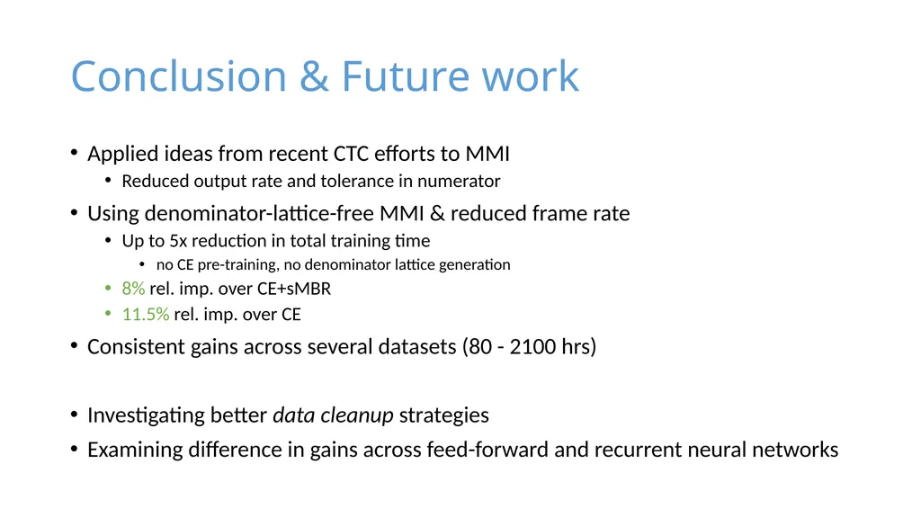
slide22. Conclusion & Future work Applied ideas from recent CTC efforts to MMI
Reduced output rate and tolerance in numerator
Using denominator-lattice-free MMI & reduced frame rate
Up to 5x reduction in total training time
no CE pre-training, no denominator lattice generation
8% rel. imp. over CE+sMBR
11.5% rel. imp. over CE
Consistent gains across several datasets (80 - 2100 hrs)
Investigating better data cleanup strategies
Examining difference in gains across feed-forward and recurrent neural networks<br>
slide2. Why should you care about this ? It gives better WERs than the conventional way of training models.
It's a lot faster to train
It's a lot faster to decode
We're modifying most of the recipes in Kaldi to use this.
Doesn't always give WER improvements on small data (e.g. < 50 hours)<br>
slide3. Connection with CTC This actually came out from some (unpublished) work on CTC.
It's a simplification of an extension of an extension of CTC.
Not really going into that work in the paper or talk. Basically I didn't see any gains with any variety of CTC (many others find this too).
Commonalities with CTC:
Objective function is posterior of the correct transcript of the utterance
30ms frame shift at the output
(see at this conf., "Lower Frame Rate NN AMs", Pundak & Sainath)<br>
slide4. What is it ? It's MMI, captain, but not as we know it.
Normally we'd do frame-by-frame training followed by MMI.
We train the neural net from a random start.
The frame shift [at the neural net output] is 30ms, not 10ms.<br>
slide5. Why is training MMI from scratch hard? In MMI training, in general there are two forward-backward algorithms, and we subtract the occupation counts (num-den)
Numerator == correct transcript
Denominator == all possible transcripts
Full forward backward or even search over denominator is slow -> must be on GPU.
On GPU, beam search is hard
Lose a lot of efficiency if different cores are taking different code paths or accessing different data<br>
slide6. How do we do it? Full forward backward of denominator
(on GPU, custom kernels)
Break up utterances into fixed-size chunks
(one-second chunks)
Keep the denominator graph small enough
so we can keep the forward (𝛼) scores on the GPU for a minibatch of utterances (e.g. 128).
In next slides, will explore the consequences of these decisions.<br>
slide7. Fixed chunk sizes Use 1-second chunks
(not highly sensitive to the exact length)
Slight overlaps or gaps where we break up utterances this way
Append successive utterances in data preparation
so all utterances are at least 1 second.
Difficulty: how do we break up the transcripts?
1-second chunks may not coincide with word boundaries.
... see next slide for solution.<br>
slide8. Numerator representation Generate a lattice for the numerator, encoding alternative pronunciations of the transcript of the original utterance.
The lattice is turned into an FST that constrains at what time the phones can appear, to +-0.05 seconds from their positions in the lattice1.
Process this into an FST whose labels are pdfs (neural-net outputs).
Extract fixed-size chunks from this FST 1. In [1], FSTs are used to constrain the labels to a certain window around where the baseline system puts them. We used the same idea here.
[1] : A. Senior, H. Sak, F. de Chaumont Quitry, T. N. Sainath, and K. Rao, “Acoustic Modelling with CD-CTC-SMBR LSTM RNNS,” in ASRU, 2015.<br>
slide9. Model topology and frame rate We use a topology that can be traversed in 1 state, and a 30ms frame shift
We did find that the 30ms frame shift was optimal for the 1-state topology.
We experimented with different topologies that can be traversed in 1 state.
Chosen topology,
Can generate "a", "ab", "abb", ...<br>
slide10. Denominator graph Denominator graph is like a decoding graph FST (HCLG).
Phone-level language model and no lexicon
so it's like HCP, where P is the phone LM.
We construct P to minimize the size of HCP.
It's a 4-gram, but with no backoff lower than 3-gram
(so that triphones not seen in training cannot be generated).
The number of states is limited by completely removing low-count 4-gram states
(backing off the counts to 3-gram).
We minimize the size of the final graph
a different-than-normal graph construction recipe<br>
slide11. Regularization Very vulnerable to over-training
Three regularization methods:
L2 regularization on the network output*
Cross-entropy regularization
Add a separate cross-entropy layer that's trained but is then thrown away (that shares the hidden layers).
"Leaky HMM".
This refers to modifying the denominator-graph so that it is "stopped and restarted" with a small probability (e.g. 0.1) on each frame [like forgetting the context].
The gains from these regularization methods are somewhat additive; we use all three (and also use smaller-than-normal models). * the outputs are in log space, they are like pseudo-likelihoods.<br>
slide12. Frame shift issues In our neural nets, the input frame shift is 10ms and the output frame shift is 30ms.
This is not quite equivalent to splicing the input, because the early TDNN and LSTM layers use frame offsets and recurrence delays that are not multiples of 30ms.
We try to keep all such frame offsets in later layers of the network as multiples of 3 so that those layers only need to be evaluated every 3 frames.
The neural network is obviously about 3 times faster to evaluate than for regular models (perhaps more, since model is smaller).
In training, on each epoch we cycle through 3 differently-shifted versions of the training data (shifted by -1, 0, 1 input frame).<br>
slide13. Speed etc. The parts of the computation that are specific to LF-MMI take less than 20% of the training time
(e.g. denominator forward-backward)
The rest is just forward-backward on the neural net.
LF-MMI training is substantially faster than conventional cross-entropy training
This due to smaller neural network and faster evaluation due to frame subsampling
We actually see the data slightly more times (slightly fewer epochs, but we duplicate the data 3-fold on each epoch).
Decoding with LF-MMI models is about 2 to 3 times faster than conventional models.<br>
slide14. Transcript Quality We initially found that this method did not work on AMI and TED-LIUM
Due to lower transcript quality (vs Switchboard, Librispeech)
The results shown in this paper for AMI are after a "fix”
We filtered out utterances that, after decoding with a biased LM, the lattice oracle path was still far from the transcript.
Since publishing this paper, we've come up with a more fine-grained data cleaning method
Bad parts of utterances are thrown away, and good parts kept.
This is a completely separate process from LF-MMI training
... but LF-MMI is particularly sensitive to its effect
We now have LF-MMI "working" on TED-LIUM (done with release 2), after this data cleanup.<br>
slide15. Left bi-phone All the results shown in this paper are with triphone models.
Typically the number of leaves is about 10% to 20% fewer than the conventional DNN system (we found this worked the best).
Since the paper was published, we've found that left biphone works *slightly* better with this type of model.
It's also faster, of course.<br>
slide16. Results<br>
slide17. Comparison of regularization functions SWBD-300 Hr task : TDNN acoustic models : HUB ‘00 eval set<br>
slide18. Comparison of LF-MMI and CE SWBD-300 Hr task : TDNN acoustic models : HUB ‘00 eval set<br>
slide19. LF-MMI with different DNNs 15 SWBD-300 Hr task
HUB ‘00 eval set<br>
slide20. LF-MMI in various LVCSR tasks TDNN acoustic models
Similar architecture across LVCSR tasks<br>
slide21. Performance of lattice-free MMI F : Fisher corpus (1800 hrs)
S: Switchboard Corpus (300 hrs)
C: Callhome corpus (14 hrs)
O: Other corpora [1] A.R.Mohamed, F.Seide, D.Yu, J.Droppo, A.Stolcke, G.Zweig and G. Penn, “Deep bi-directional recurrent networks over spectral windows,” in Proceedings of ASRU. ASRU, 2015.
[2] G. Saon, H.K. J. Kuo, S. Rennie, and M. Picheny, “The IBM 2015 English Conversational Telephone Speech Recognition System,” 2015. Available: http://arxiv.org/abs/ 1505.05899
*Better results reported in Saon et. al., “The IBM 2016 English Conversational Telephone Speech Recognition System”, this conf.<br>
slide22. Conclusion & Future work Applied ideas from recent CTC efforts to MMI
Reduced output rate and tolerance in numerator
Using denominator-lattice-free MMI & reduced frame rate
Up to 5x reduction in total training time
no CE pre-training, no denominator lattice generation
8% rel. imp. over CE+sMBR
11.5% rel. imp. over CE
Consistent gains across several datasets (80 - 2100 hrs)
Investigating better data cleanup strategies
Examining difference in gains across feed-forward and recurrent neural networks<br>