Radiative Transfer & Volume Path Tracing CS295,

slide1. Radiative Transfer & Volume Path Tracing CS295, Spring 2017
Shuang Zhao Computer Science Department University of California, Irvine

Modified from the original slides CS295, Spring 2017 Shuang Zhao 1<br>
slide2. CS295, Spring 2017 Shuang Zhao 2 Today’s Lecture Radiative transfer
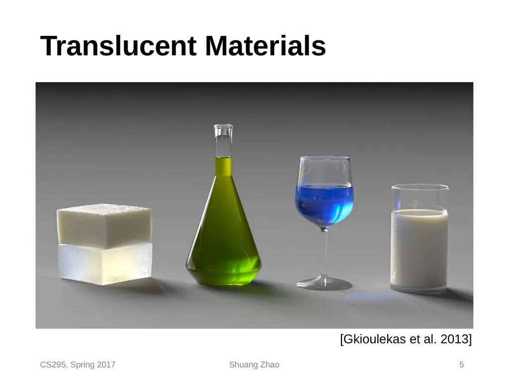
The mathematical model to simulate light scattering in participating media (e.g., smoke) and translucent materials (e.g., marble and skin)

Volume path tracing (VPT)
A Monte Carlo solution to the radiative transfer problem
Similar to the normal PT from previous lectures<br>
slide3. CS295, Spring 2017 Shuang Zhao 3 Radiative Transfer CS295: Realistic Image Synthesis<br>
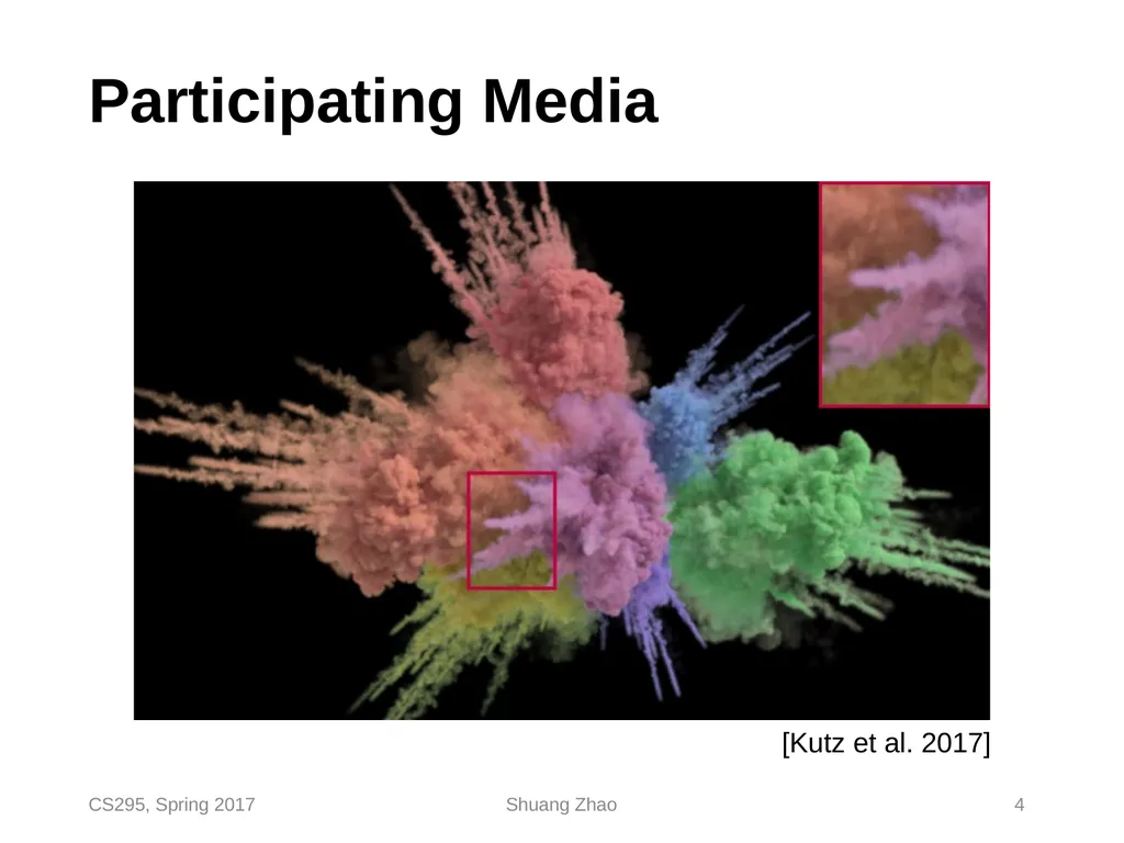
slide4. Participating Media [Kutz et al. 2017] CS295, Spring 2017 Shuang Zhao 4<br>
slide5. Translucent Materials [Gkioulekas et al. 2013] CS295, Spring 2017 Shuang Zhao 5<br>
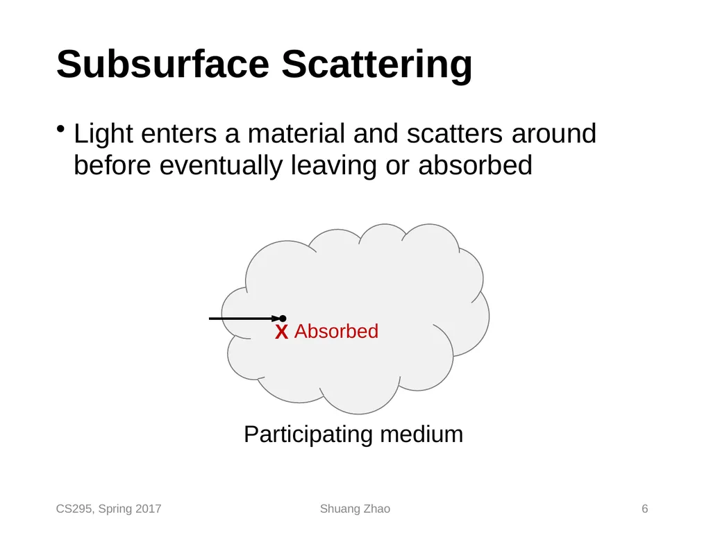
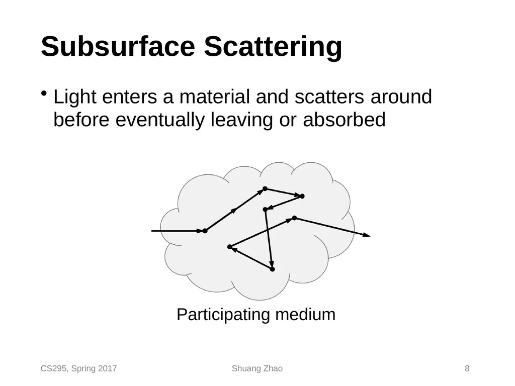
slide6. Subsurface Scattering Light enters a material and scatters around
before eventually leaving or absorbed X Absorbed CS295, Spring 2017 Shuang Zhao 6 Participating medium<br>
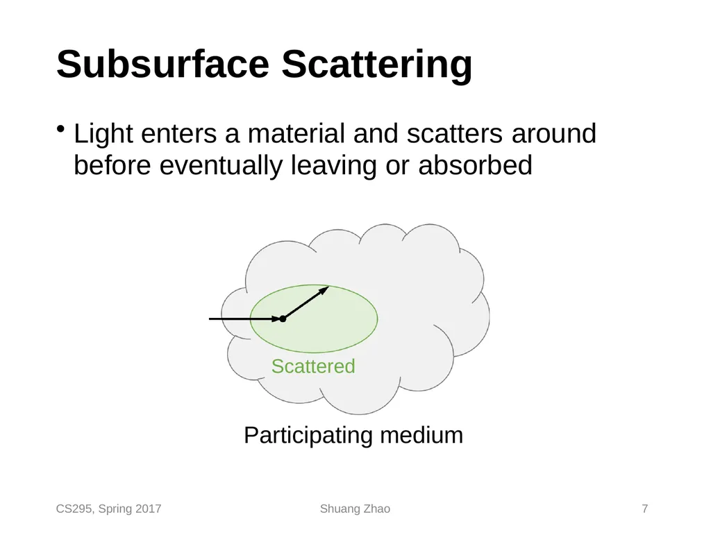
slide7. Subsurface Scattering Light enters a material and scatters around
before eventually leaving or absorbed Scattered

Participating medium CS295, Spring 2017 Shuang Zhao 7<br>
slide8. Subsurface Scattering Light enters a material and scatters around
before eventually leaving or absorbed Participating medium CS295, Spring 2017 Shuang Zhao 8<br>
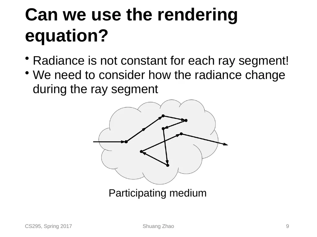
slide9. Can we use the rendering equation? Radiance is not constant for each ray segment!
We need to consider how the radiance change during the ray segment Participating medium CS295, Spring 2017 Shuang Zhao 9<br>
slide10. CS295, Spring 2017 Shuang Zhao 10 Radiative Transfer A mathematical model describing how light
interacts with participating media
Originated in physics
Now used in many areas
Astrophysics (light transport in space)
Biomedicine (light transport in human tissue)
Graphics
Nuclear science & engineering (neutron transport)
Remote sensing
…<br>
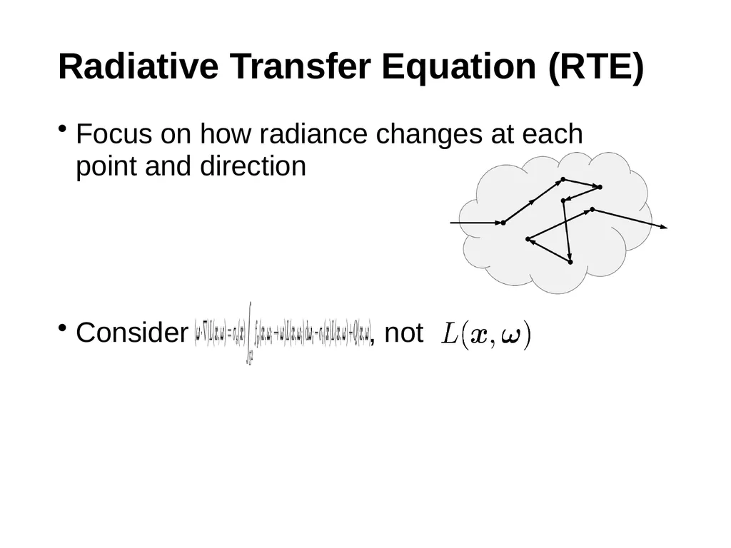
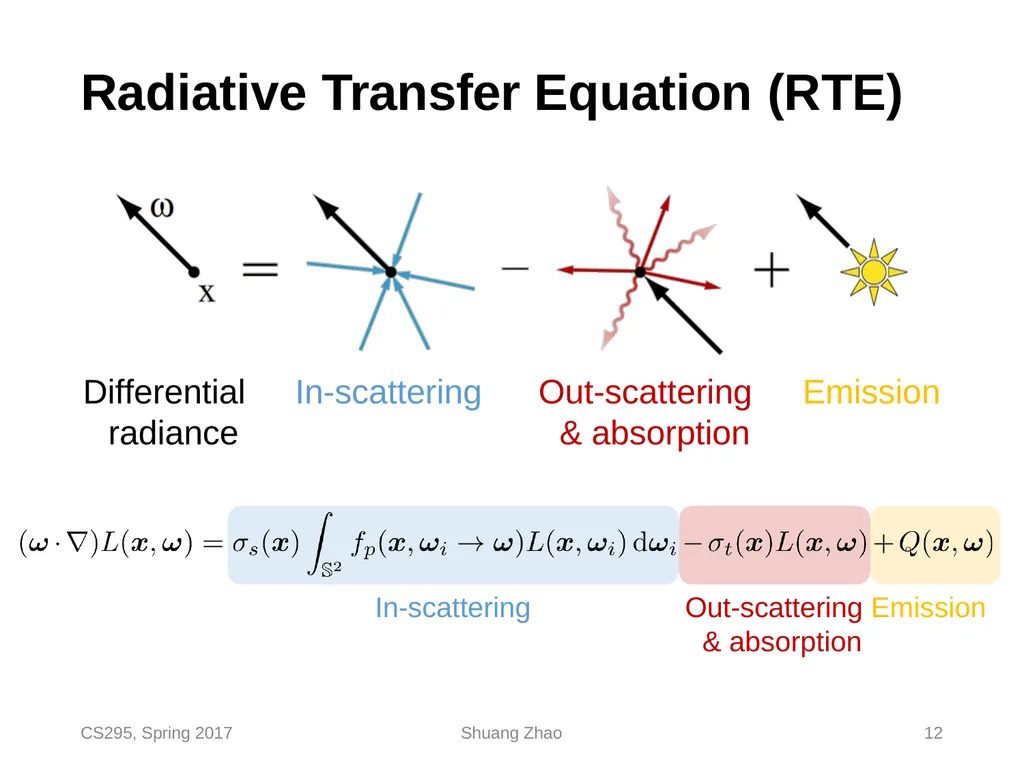
slide11. Radiative Transfer Equation (RTE) Focus on how radiance changes at each point and direction

Consider , not<br>
slide12. Radiative Transfer Equation (RTE) In-scattering Out-scattering & absorption Emission Differential radiance In-scattering CS295, Spring 2017 Shuang Zhao 12 Out-scattering Emission & absorption<br>
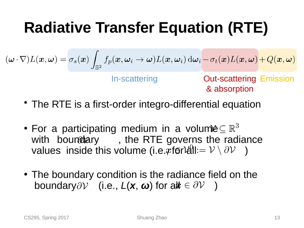
slide13. Radiative Transfer Equation (RTE) The RTE is a first-order integro-differential equation

For a participating medium in a volume with boundary , the RTE governs the radiance values inside this volume (i.e., for all )

The boundary condition is the radiance field on the boundary (i.e., L(x, ω) for all ) In-scattering Out-scattering Emission
& absorption CS295, Spring 2017 Shuang Zhao 13<br>
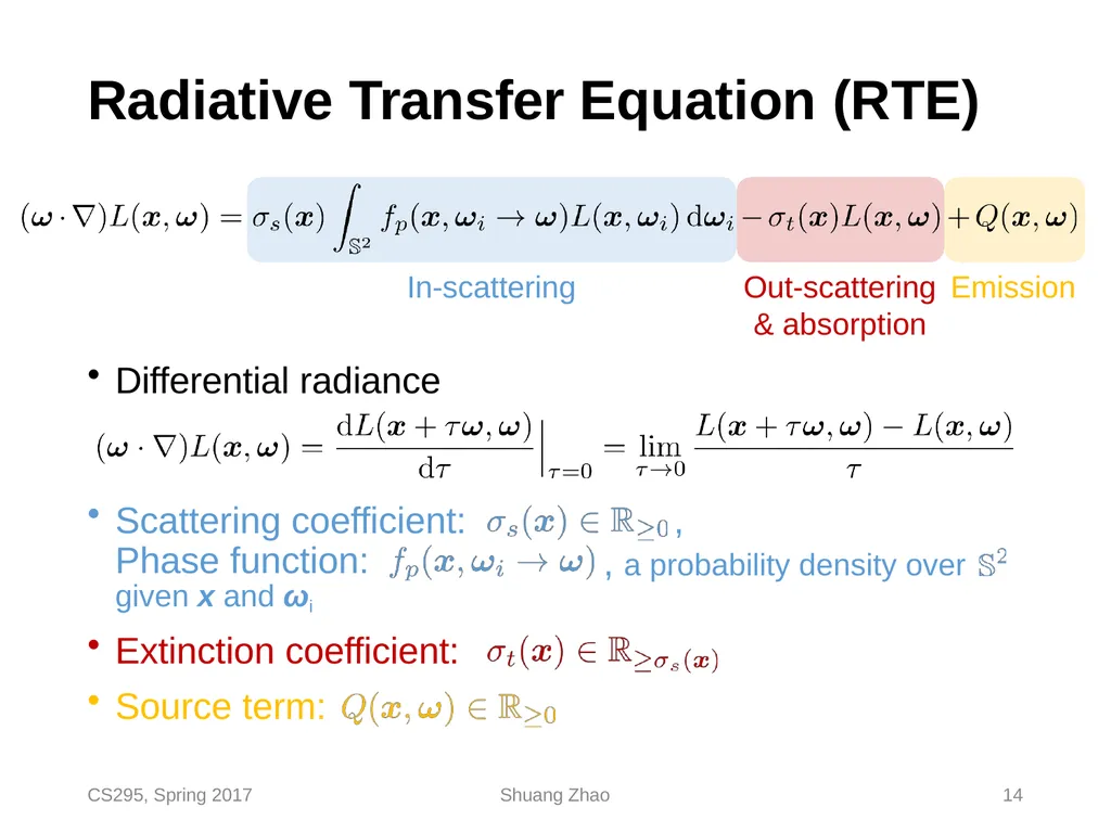
slide14. Radiative Transfer Equation (RTE) Differential radiance ,
, a probability density over Scattering coefficient:
Phase function:
given x and ωi
Extinction coefficient:
Source term: In-scattering Out-scattering Emission
& absorption CS295, Spring 2017 Shuang Zhao 14<br>
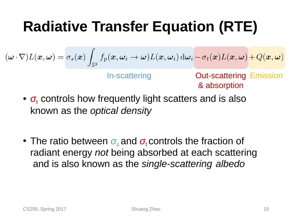
slide15. Radiative Transfer Equation (RTE) σt controls how frequently light scatters and is also
known as the optical density

The ratio between σs and σt controls the fraction of radiant energy not being absorbed at each scattering and is also known as the single-scattering albedo In-scattering CS295, Spring 2017 Shuang Zhao 15 Out-scattering Emission
& absorption<br>
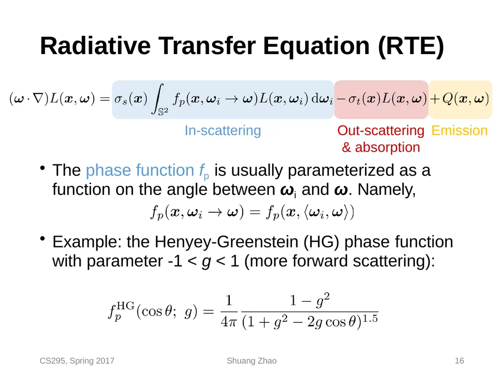
slide16. Radiative Transfer Equation (RTE) The phase function fp is usually parameterized as a
function on the angle between ωi and ω. Namely,

Example: the Henyey-Greenstein (HG) phase function
with parameter -1 < g < 1 (more forward scattering): In-scattering Out-scattering Emission
& absorption CS295, Spring 2017 Shuang Zhao 16<br>
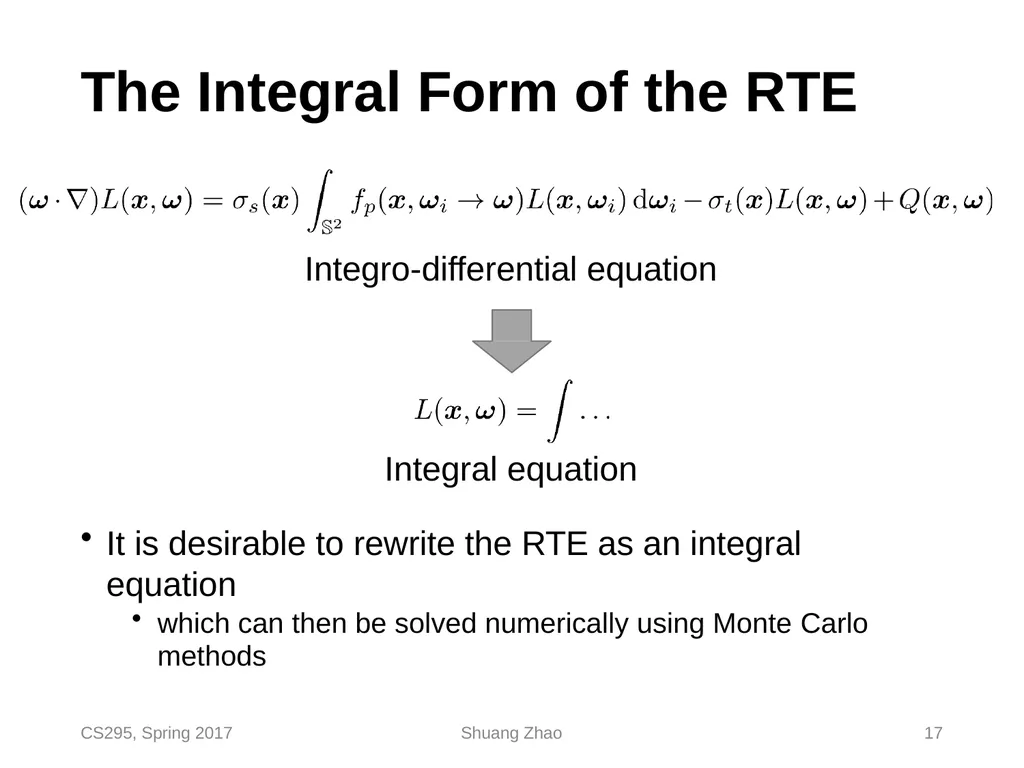
slide17. The Integral Form of the RTE Integro-differential equation Integral equation
It is desirable to rewrite the RTE as an integral equation
which can then be solved numerically using Monte Carlo
methods CS295, Spring 2017 Shuang Zhao 17<br>
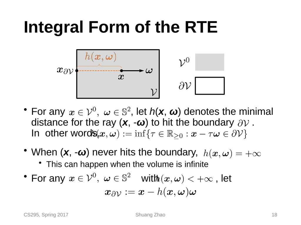
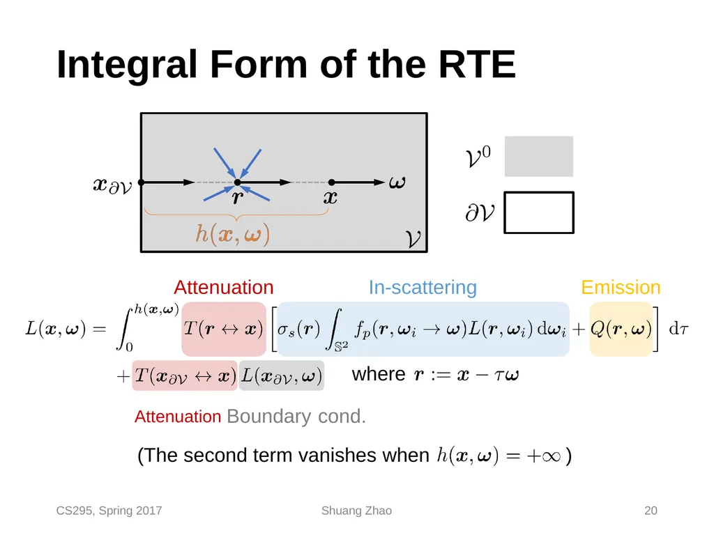
slide18. Integral Form of the RTE For any , let h(x, ω) denotes the minimal distance for the ray (x, -ω) to hit the boundary . In other words, When (x, -ω) never hits the boundary,
This can happen when the volume is infinite
For any with , let CS295, Spring 2017 Shuang Zhao 18<br>
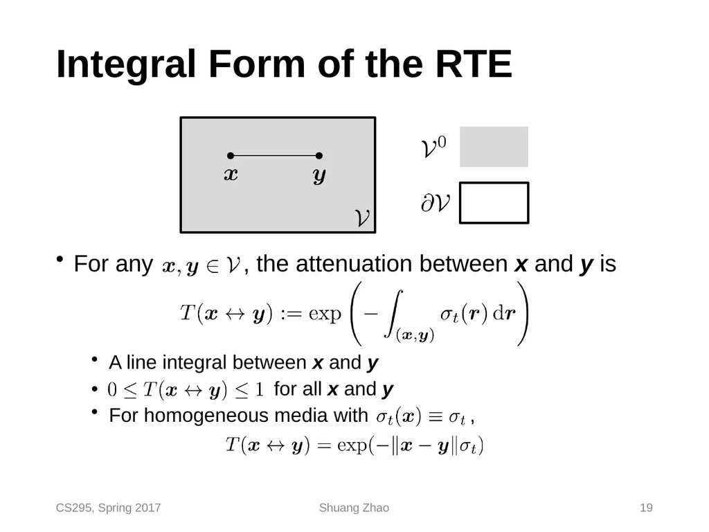
slide19. Integral Form of the RTE For any , the attenuation between x and y is A line integral between x and y • for all x and y For homogeneous media with , CS295, Spring 2017 Shuang Zhao 19<br>
slide20. Integral Form of the RTE In-scattering Emission Attenuation (The second term vanishes when ) where
Attenuation Boundary cond. CS295, Spring 2017 Shuang Zhao 20<br>
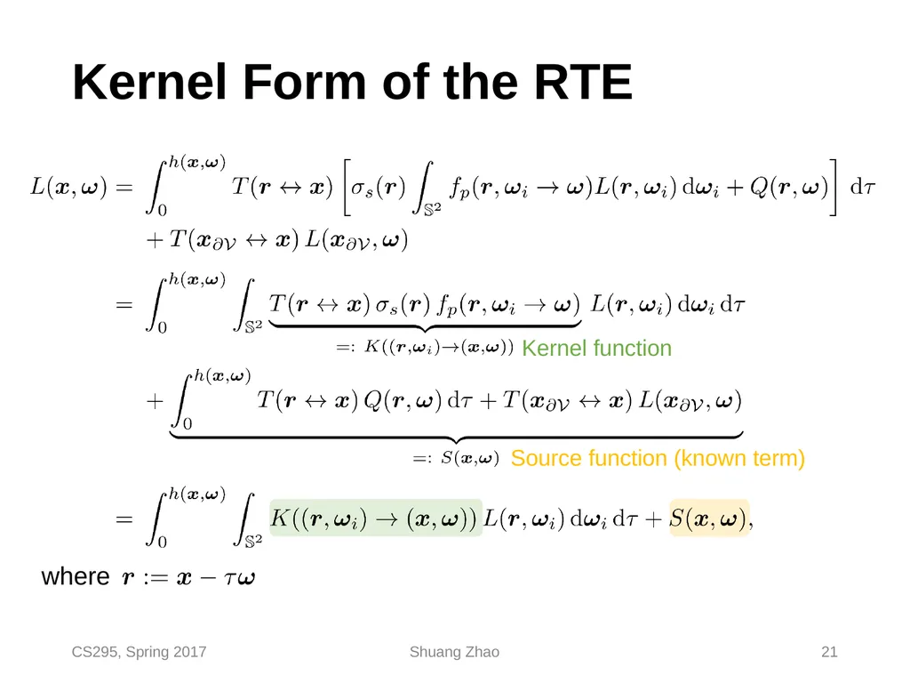
slide21. Kernel Form of the RTE where Kernel function CS295, Spring 2017 Shuang Zhao 21 Source function (known term)<br>
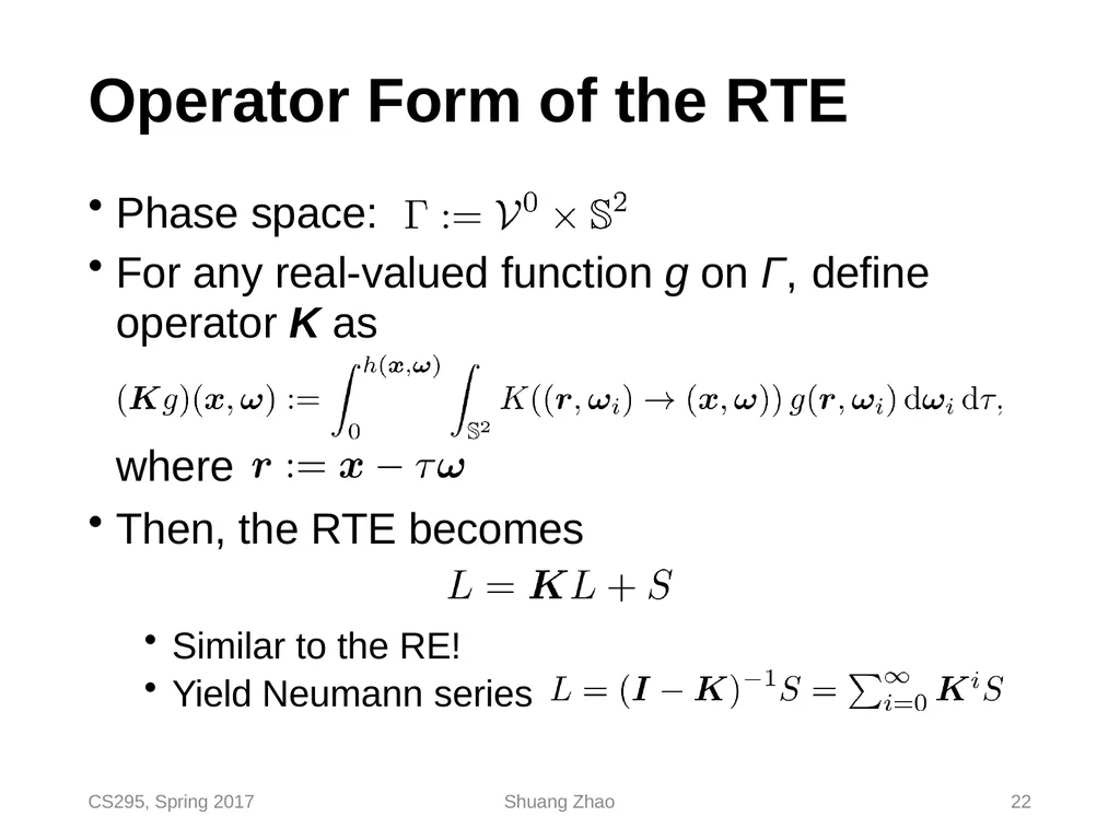
slide22. Operator Form of the RTE Phase space:
For any real-valued function g on Γ, define
operator K as

where
Then, the RTE becomes

Similar to the RE!
Yield Neumann series CS295, Spring 2017 Shuang Zhao 22<br>
slide23. CS295, Spring 2017 Shuang Zhao 23 Volume Path Tracing CS295: Realistic Image Synthesis Start from here…<br>
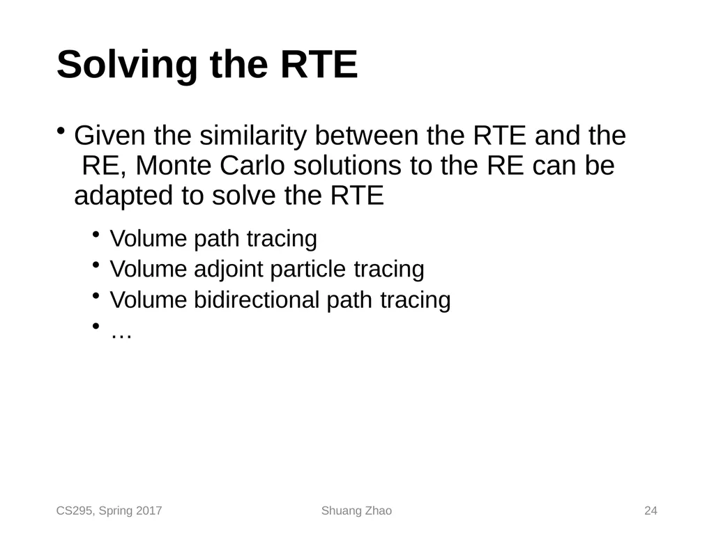
slide24. CS295, Spring 2017 Shuang Zhao 24 Solving the RTE Given the similarity between the RTE and the RE, Monte Carlo solutions to the RE can be adapted to solve the RTE
Volume path tracing
Volume adjoint particle tracing
Volume bidirectional path tracing
…<br>
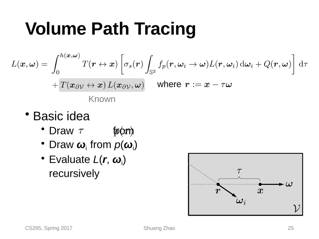
slide25. Volume Path Tracing where
Known
Basic idea
Draw from
Draw ωi from p(ωi)
Evaluate L(r, ωi) recursively CS295, Spring 2017 Shuang Zhao 25<br>
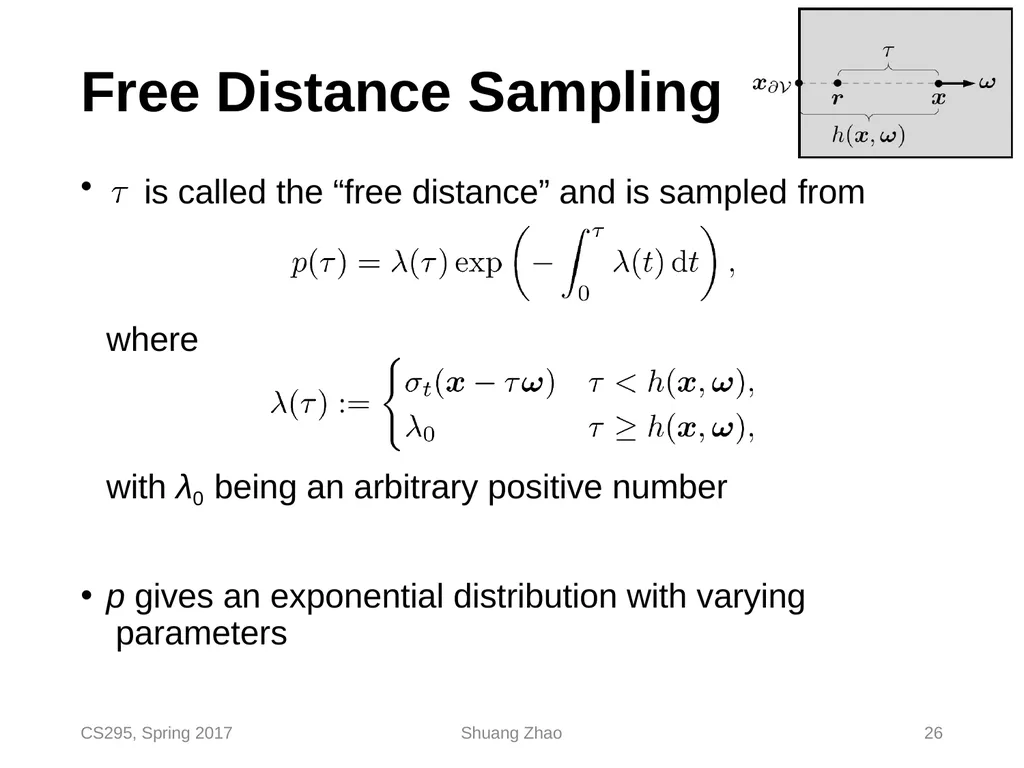
slide26. Free Distance Sampling is called the “free distance” and is sampled from where with λ0 being an arbitrary positive number

p gives an exponential distribution with varying parameters CS295, Spring 2017 Shuang Zhao 26<br>
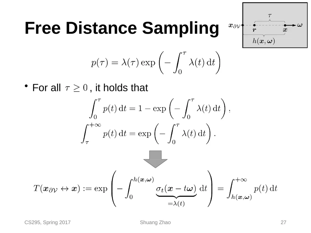
slide27. Free Distance Sampling For all , it holds that CS295, Spring 2017 Shuang Zhao 27<br>
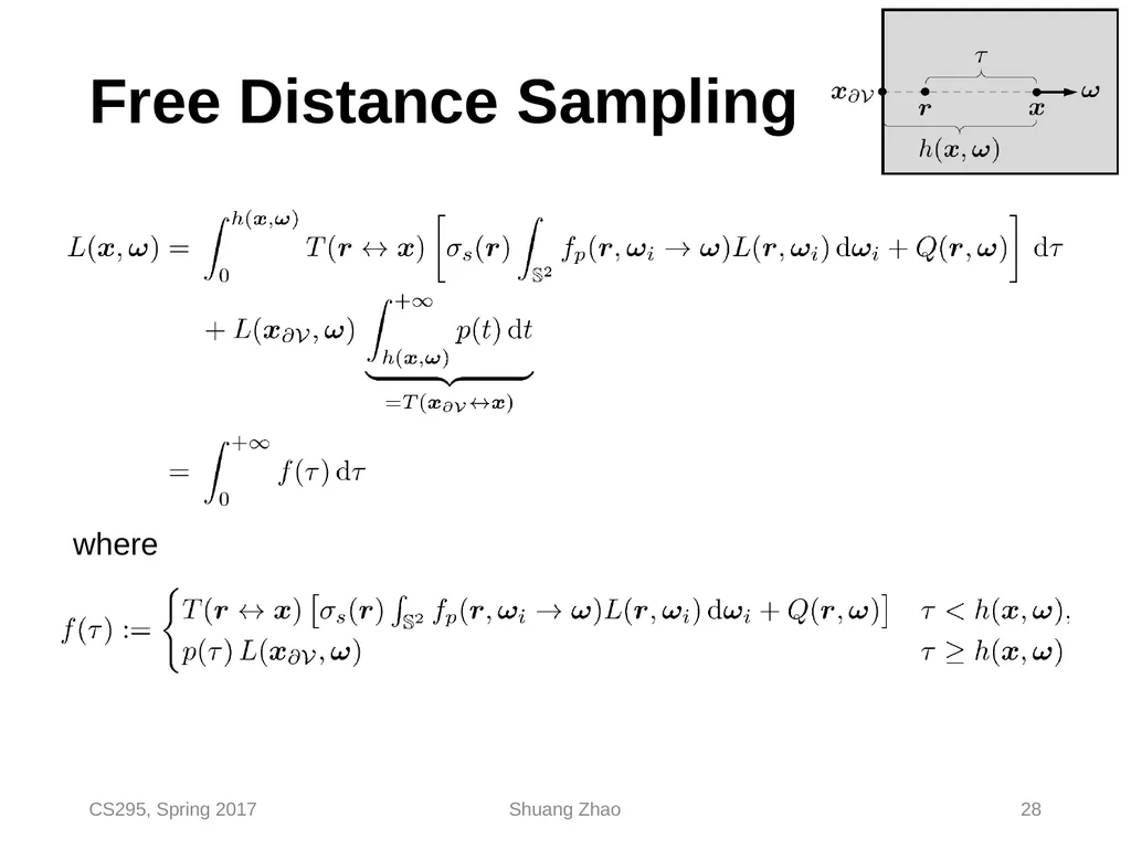
slide28. Free Distance Sampling where CS295, Spring 2017 Shuang Zhao 28<br>
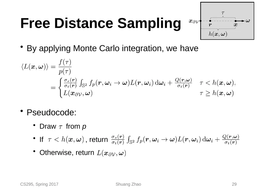
slide29. Free Distance Sampling By applying Monte Carlo integration, we have Pseudocode: Draw
If from p
, return Otherwise, return CS295, Spring 2017 Shuang Zhao 29<br>
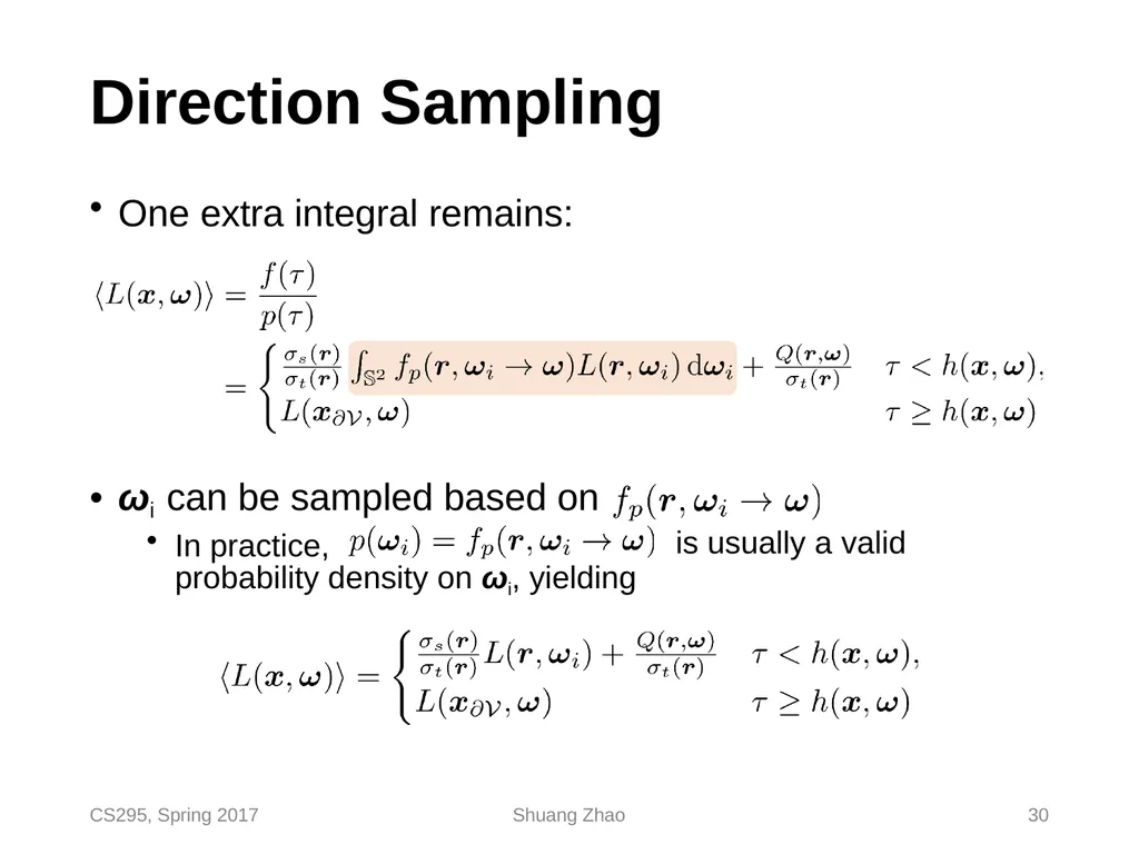
slide30. Direction Sampling One extra integral remains: is usually a valid ωi can be sampled based on
In practice,
probability density on ωi, yielding CS295, Spring 2017 Shuang Zhao 30<br>
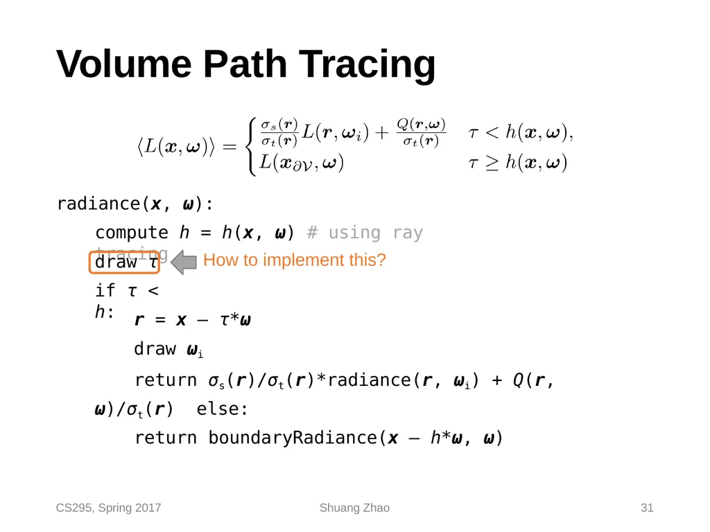
slide31. Volume Path Tracing radiance(x, ω):
compute h = h(x, ω) # using ray tracing draw τ
if τ < h: r = x – τ*ω
draw ωi
return σs(r)/σt(r)*radiance(r, ωi) + Q(r, ω)/σt(r) else:
return boundaryRadiance(x – h*ω, ω) How to implement this? CS295, Spring 2017 Shuang Zhao 31<br>
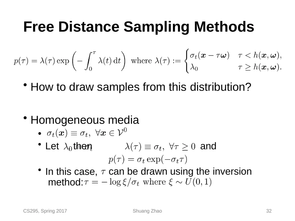
slide32. Free Distance Sampling Methods How to draw samples from this distribution? Homogeneous media
•
Let , then and can be drawn using the inversion In this case, method: CS295, Spring 2017 Shuang Zhao 32<br>
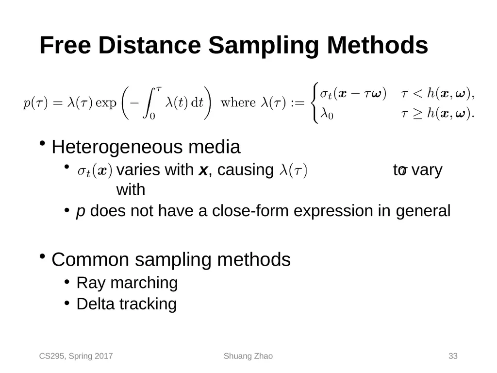
slide33. Free Distance Sampling Methods Heterogeneous media
varies with x, causing to vary with
p does not have a close-form expression in general

Common sampling methods
Ray marching
Delta tracking CS295, Spring 2017 Shuang Zhao 33<br>
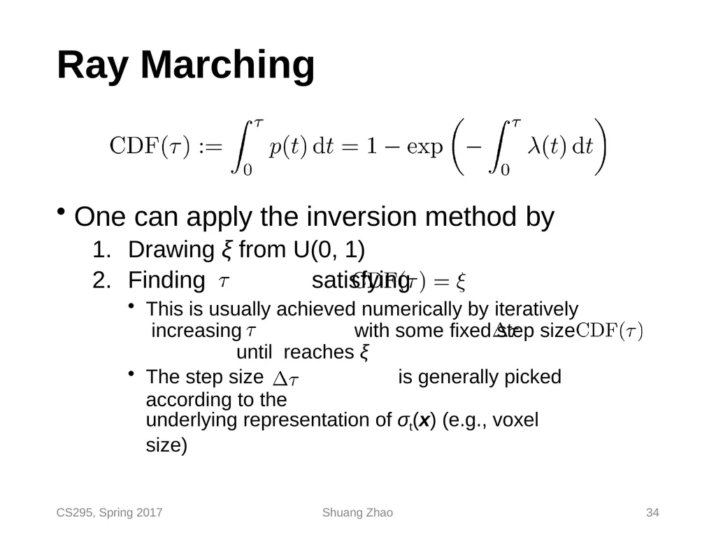
slide34. Ray Marching One can apply the inversion method by
Drawing ξ from U(0, 1)
Finding satisfying
This is usually achieved numerically by iteratively increasing with some fixed step size until reaches ξ
The step size is generally picked according to the
underlying representation of σt(x) (e.g., voxel size) CS295, Spring 2017 Shuang Zhao 34<br>
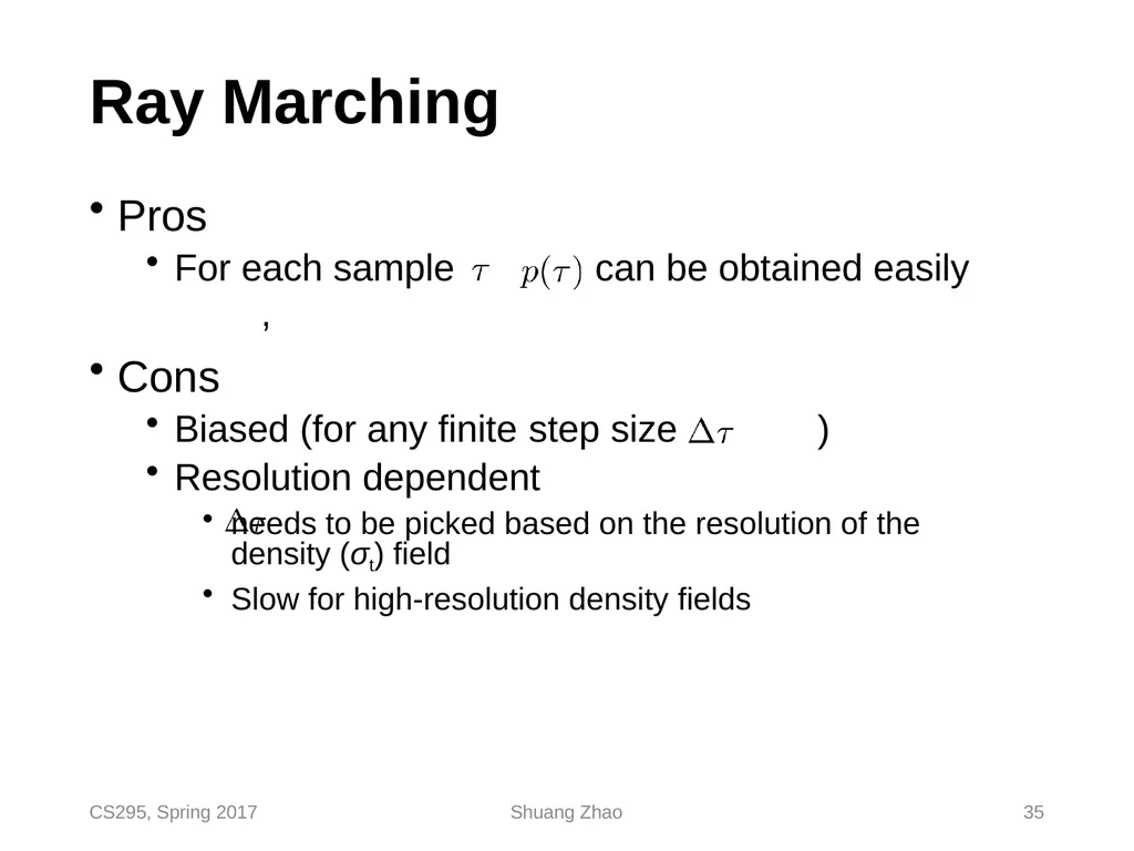
slide35. Ray Marching Pros
For each sample , can be obtained easily Cons
Biased (for any finite step size )
Resolution dependent
needs to be picked based on the resolution of the density (σt) field
Slow for high-resolution density fields CS295, Spring 2017 Shuang Zhao 35<br>
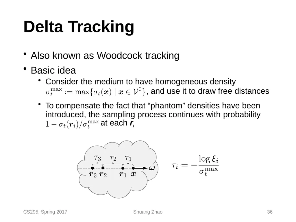
slide36. Delta Tracking Also known as Woodcock tracking
Basic idea
Consider the medium to have homogeneous density
, and use it to draw free distances
To compensate the fact that “phantom” densities have been
introduced, the sampling process continues with probability
at each ri CS295, Spring 2017 Shuang Zhao 36<br>
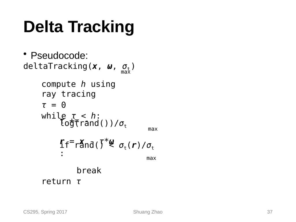
slide37. CS295, Spring 2017 Shuang Zhao 37 Delta Tracking Pseudocode:
deltaTracking(x, ω, σt )
max
compute h using ray tracing
τ = 0
while τ < h:
τ += -log(rand())/σt
max
r = x - τ*ω
if rand() < σt(r)/σt :
max
break
return τ<br>
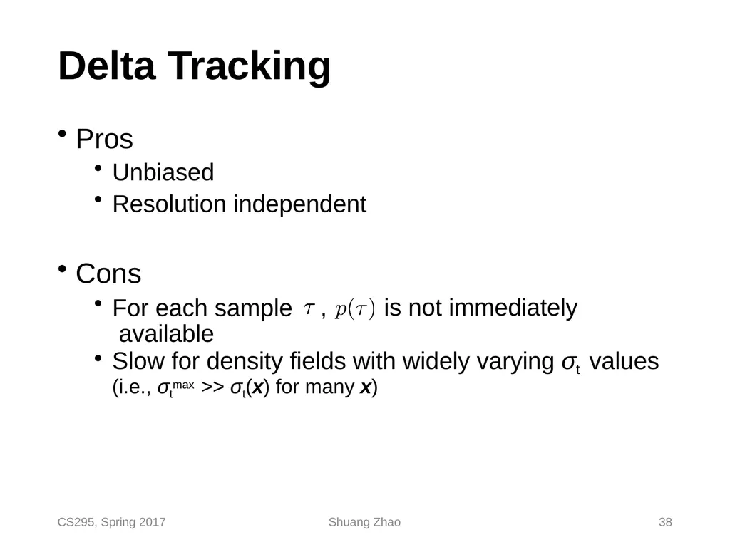
slide38. Delta Tracking Pros
Unbiased
Resolution independent , is not immediately Cons
For each sample available Slow for density fields with widely varying σt values
(i.e., σtmax >> σt(x) for many x) CS295, Spring 2017 Shuang Zhao 38<br>
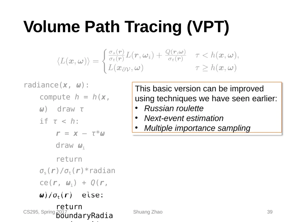
slide39. Volume Path Tracing (VPT) radiance(x, ω):
compute h = h(x, ω) draw τ
if τ < h:
r = x – τ*ω
draw ωi
return σs(r)/σt(r)*radiance(r, ωi) + Q(r, ω)/σt(r) else:
return boundaryRadiance(x – h*ω, ω) This basic version can be improved using techniques we have seen earlier:
Russian roulette
Next-event estimation
Multiple importance sampling CS295, Spring 2017 Shuang Zhao 39<br>
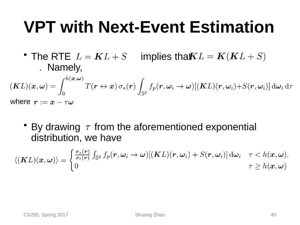
slide40. VPT with Next-Event Estimation The RTE implies that . Namely, By drawing from the aforementioned exponential distribution, we have where CS295, Spring 2017 Shuang Zhao 40<br>
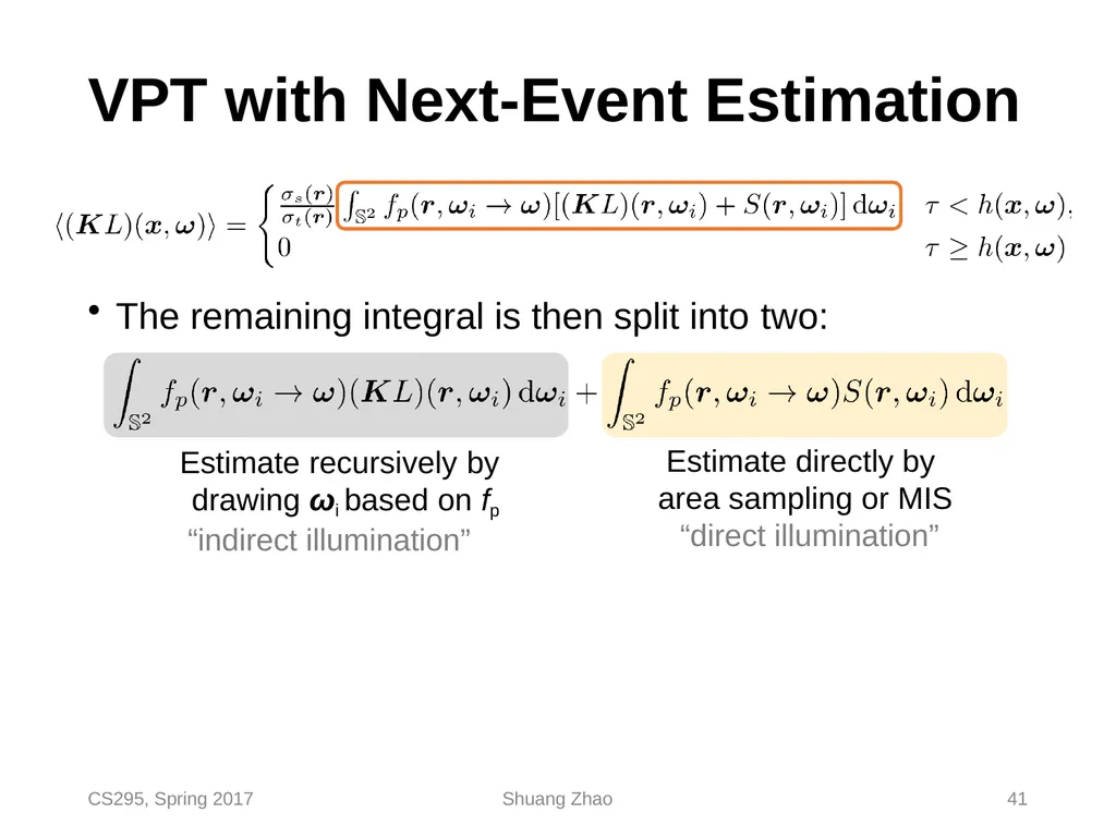
slide41. VPT with Next-Event Estimation The remaining integral is then split into two: Estimate recursively by drawing ωi based on fp “indirect illumination” Estimate directly by area sampling or MIS “direct illumination” CS295, Spring 2017 Shuang Zhao 41<br>
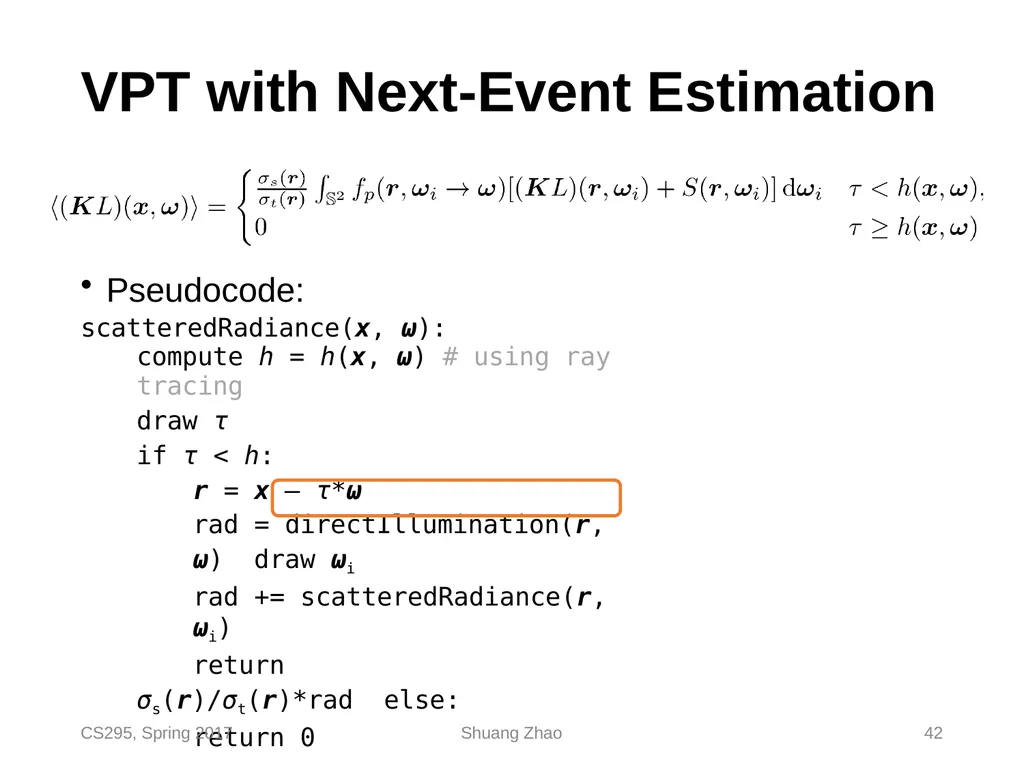
slide42. VPT with Next-Event Estimation Pseudocode:
scatteredRadiance(x, ω):
compute h = h(x, ω) # using ray tracing
draw τ
if τ < h:
r = x – τ*ω
rad = directIllumination(r, ω) draw ωi
rad += scatteredRadiance(r, ωi)
return σs(r)/σt(r)*rad else:
return 0 CS295, Spring 2017 Shuang Zhao 42<br>
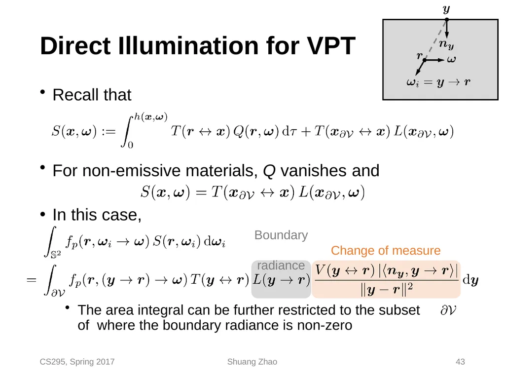
slide43. Direct Illumination for VPT Recall that For non-emissive materials, Q vanishes and

In this case, The area integral can be further restricted to the subset of where the boundary radiance is non-zero Change of measure Boundary radiance CS295, Spring 2017 Shuang Zhao 43<br>
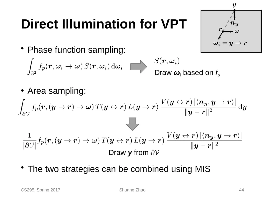
slide44. Direct Illumination for VPT Phase function sampling:

Draw ωi based on fp
Area sampling: Draw y from
The two strategies can be combined using MIS CS295, Spring 2017 Shuang Zhao 44<br>