
Random Walks and Markov Chains Nimantha Thushan
LO
Published · 90 slides · 0 views

1 / 1









Description
Random Walks and Markov Chains Nimantha Thushan Baranasuriya Girisha Durrel De Silva Rahul Singhal Karthik Yadati Ziling Zhou Outline Random Walks Markov Chains Applications 2SAT 3SAT Card Shuffling Random Walks A typical random walk
Related Topics
Share
Embed code
Download this presentation From Below
"Random Walks and Markov Chains Nimantha Thushan" is the property of its rightful owner. Permission is granted to download and print the materials on this website for personal, non-commercial use only, and to display it on your personal computer provided you do not modify the materials and that you retain all copyright notices contained in the materials. By downloading content from our website, you accept the terms of this agreement.
Presentation Transcript
01
Random Walks and Markov Chains Nimantha Thushan Baranasuriya
Girisha Durrel De Silva
Rahul Singhal
Karthik Yadati
Ziling Zhou<br>
Girisha Durrel De Silva
Rahul Singhal
Karthik Yadati
Ziling Zhou<br>
02
Outline Random Walks
Markov Chains
Applications
2SAT
3SAT
Card Shuffling<br>
Markov Chains
Applications
2SAT
3SAT
Card Shuffling<br>
03
Random Walks<br>
04
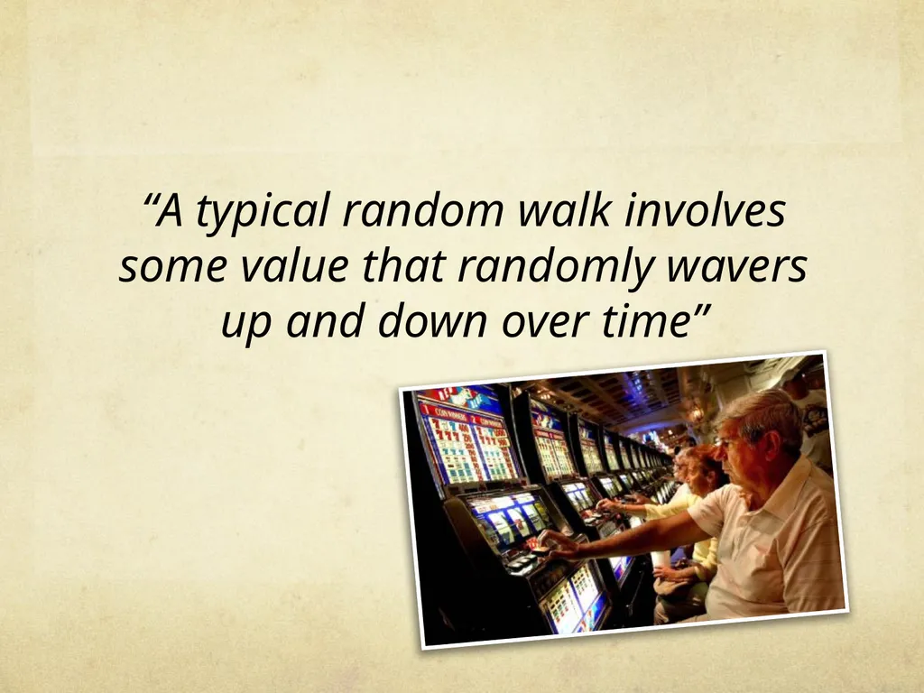
“A typical random walk involves some value that randomly wavers up and down over time”<br>
05
Commonly Analyzed Probability that the wavering value reaches some end-value
The time it takes for that to happen<br>
The time it takes for that to happen<br>
06
Uses<br>
07
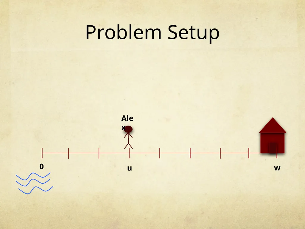
The Drunkard’s Problem Will he go home or end up in the river?<br>
08
Problem Setup<br>
09
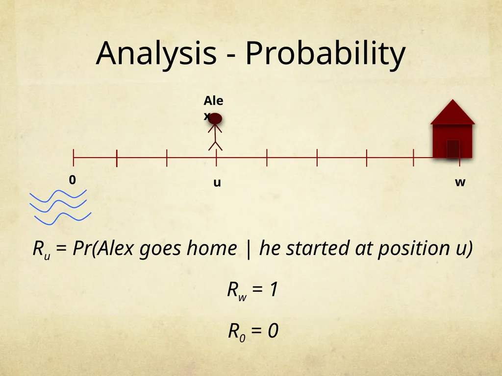
Analysis - Probability Ru = Pr(Alex goes home | he started at position u)
Rw = 1
R0 = 0<br>
Rw = 1
R0 = 0<br>
10
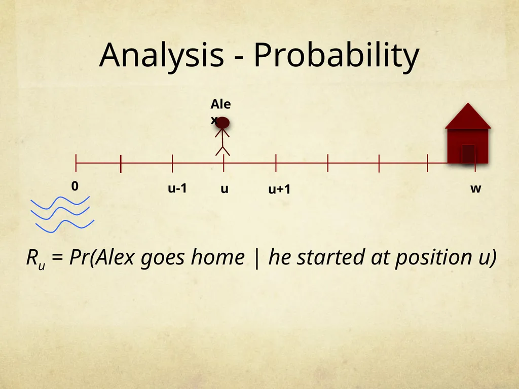
Analysis - Probability Ru = Pr(Alex goes home | he started at position u) 0 u w Alex u-1 u+1<br>
11
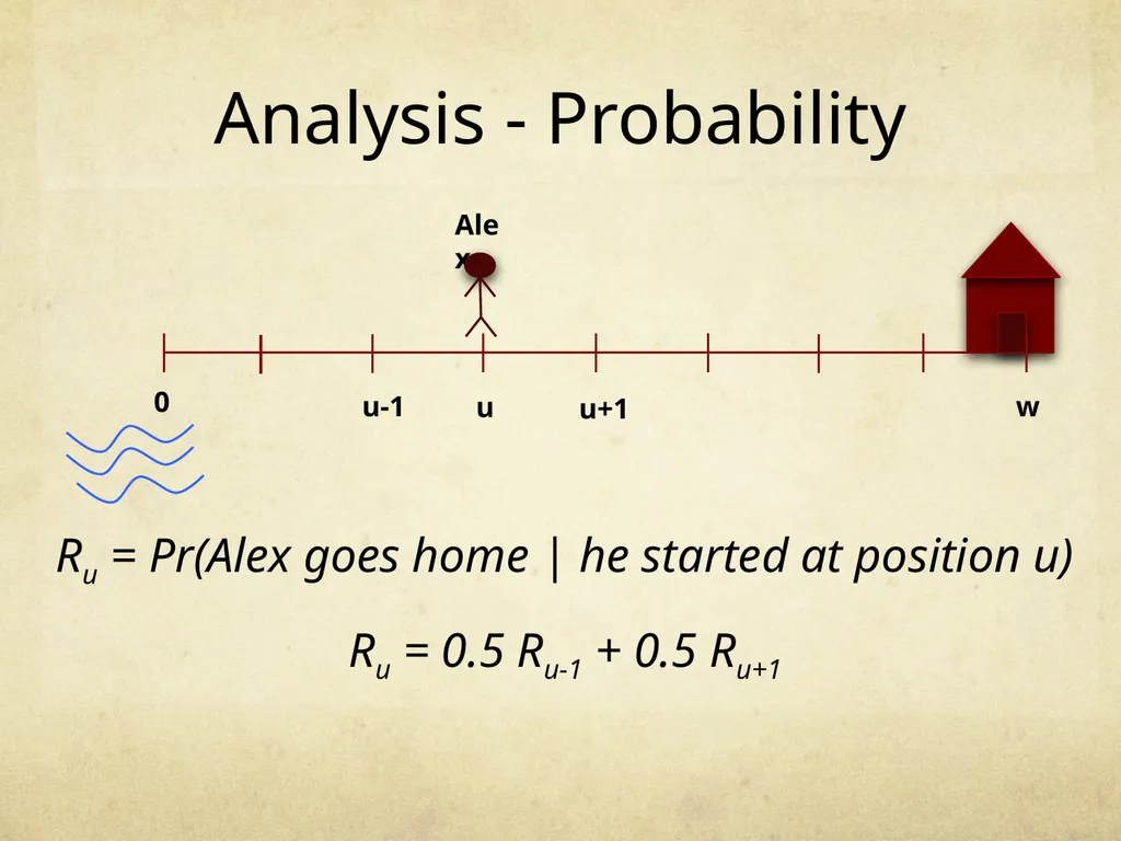
Analysis - Probability Ru = Pr(Alex goes home | he started at position u)
Ru = 0.5 Ru-1 + 0.5 Ru+1 0 u w Alex u-1 u+1<br>
Ru = 0.5 Ru-1 + 0.5 Ru+1 0 u w Alex u-1 u+1<br>
12
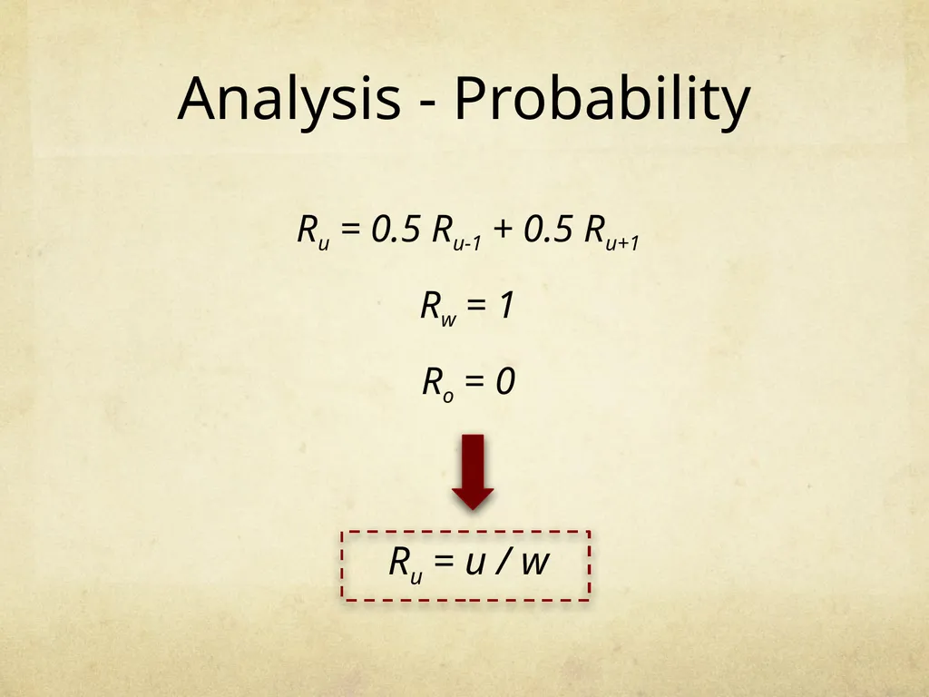
Analysis - Probability Ru = 0.5 Ru-1 + 0.5 Ru+1
Rw = 1
Ro = 0 Ru = u / w<br>
Rw = 1
Ro = 0 Ru = u / w<br>
13
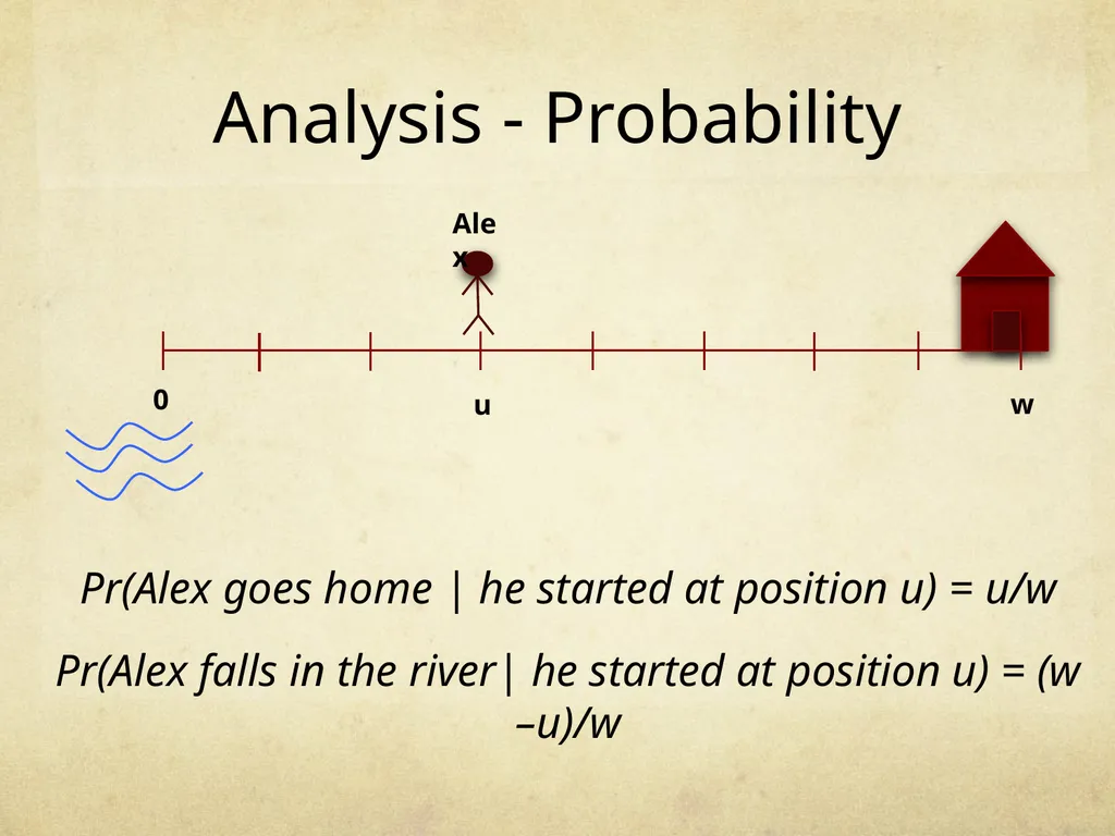
Analysis - Probability Pr(Alex goes home | he started at position u) = u/w
Pr(Alex falls in the river| he started at position u) = (w –u)/w<br>
Pr(Alex falls in the river| he started at position u) = (w –u)/w<br>
14
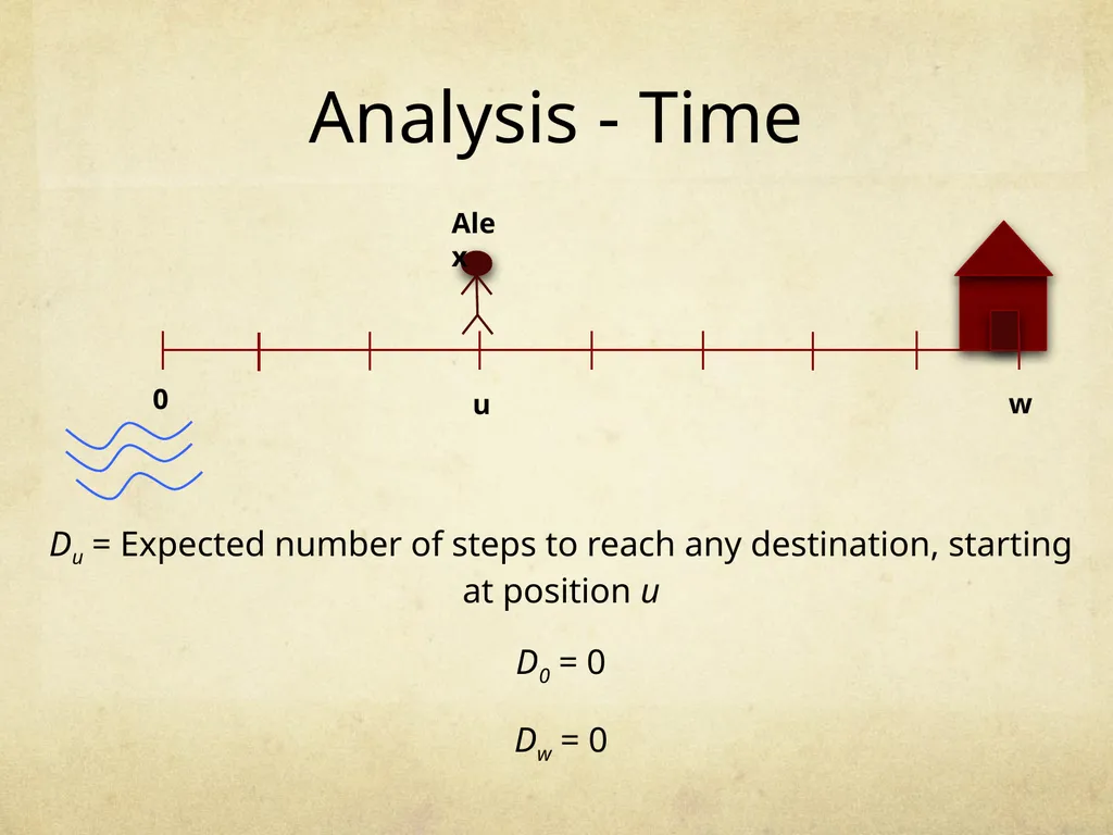
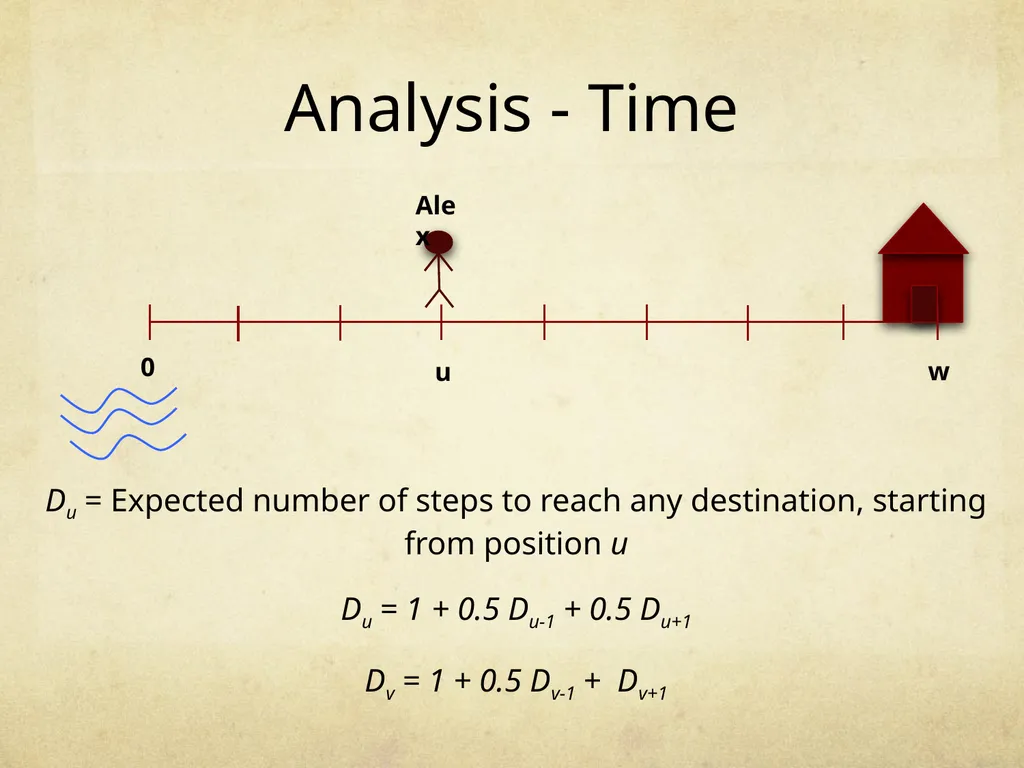
Analysis - Time Du = Expected number of steps to reach any destination, starting at position u
D0 = 0
Dw = 0<br>
D0 = 0
Dw = 0<br>
15
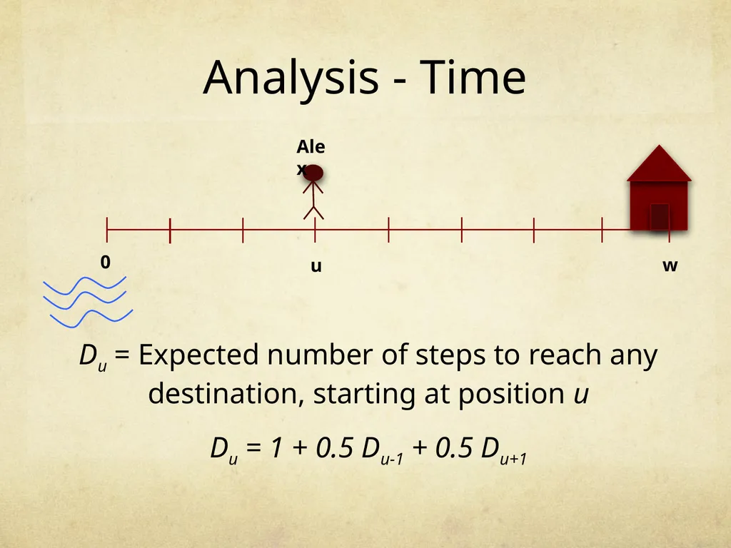
Analysis - Time Du = Expected number of steps to reach any destination, starting at position u
Du = 1 + 0.5 Du-1 + 0.5 Du+1<br>
Du = 1 + 0.5 Du-1 + 0.5 Du+1<br>
16
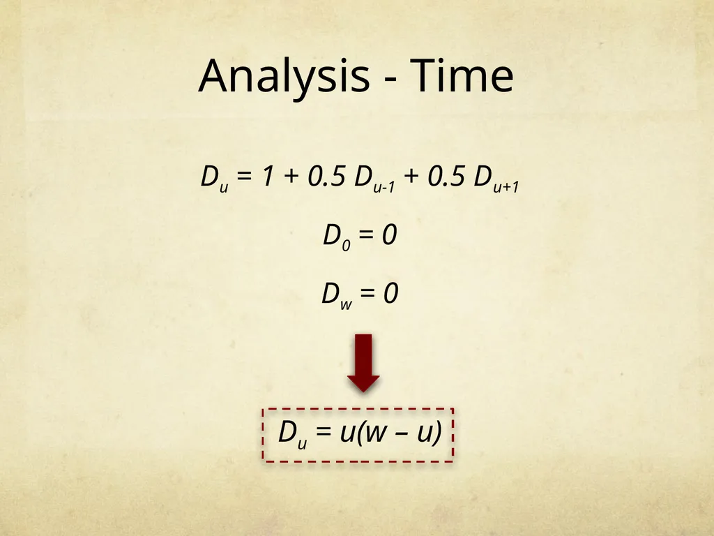
Analysis - Time Du = 1 + 0.5 Du-1 + 0.5 Du+1
D0 = 0
Dw = 0 Du = u(w – u)<br>
D0 = 0
Dw = 0 Du = u(w – u)<br>
17
Markov Chains<br>
18
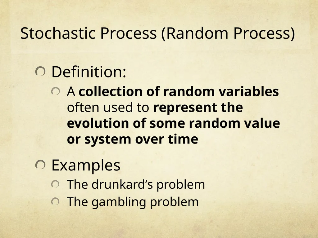
Stochastic Process (Random Process) Definition:
A collection of random variables often used to represent the evolution of some random value or system over time
Examples
The drunkard’s problem
The gambling problem<br>
A collection of random variables often used to represent the evolution of some random value or system over time
Examples
The drunkard’s problem
The gambling problem<br>
19
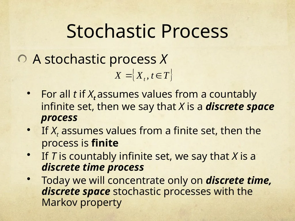
Stochastic Process A stochastic process X For all t if Xt assumes values from a countably infinite set, then we say that X is a discrete space process
If Xt assumes values from a finite set, then the process is finite
If T is countably infinite set, we say that X is a discrete time process
Today we will concentrate only on discrete time, discrete space stochastic processes with the Markov property<br>
If Xt assumes values from a finite set, then the process is finite
If T is countably infinite set, we say that X is a discrete time process
Today we will concentrate only on discrete time, discrete space stochastic processes with the Markov property<br>
20
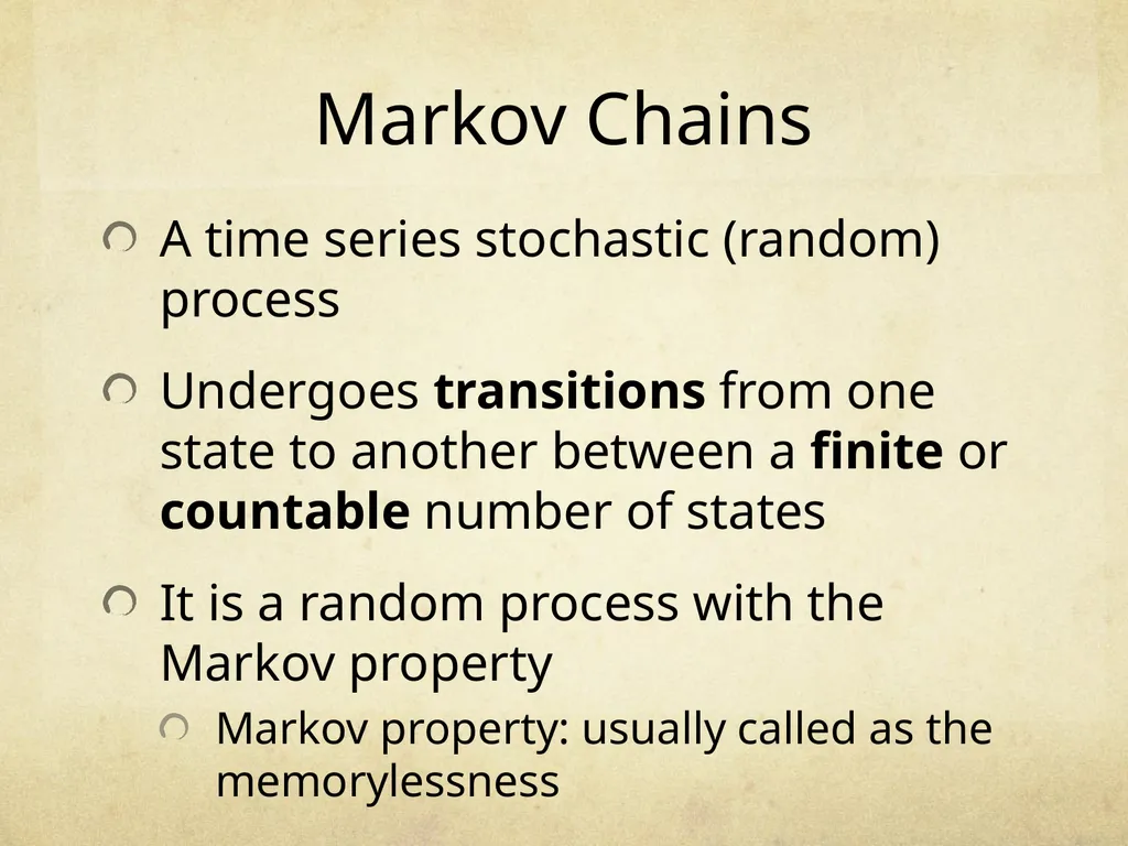
Markov Chains A time series stochastic (random) process
Undergoes transitions from one state to another between a finite or countable number of states
It is a random process with the Markov property
Markov property: usually called as the memorylessness<br>
Undergoes transitions from one state to another between a finite or countable number of states
It is a random process with the Markov property
Markov property: usually called as the memorylessness<br>
21
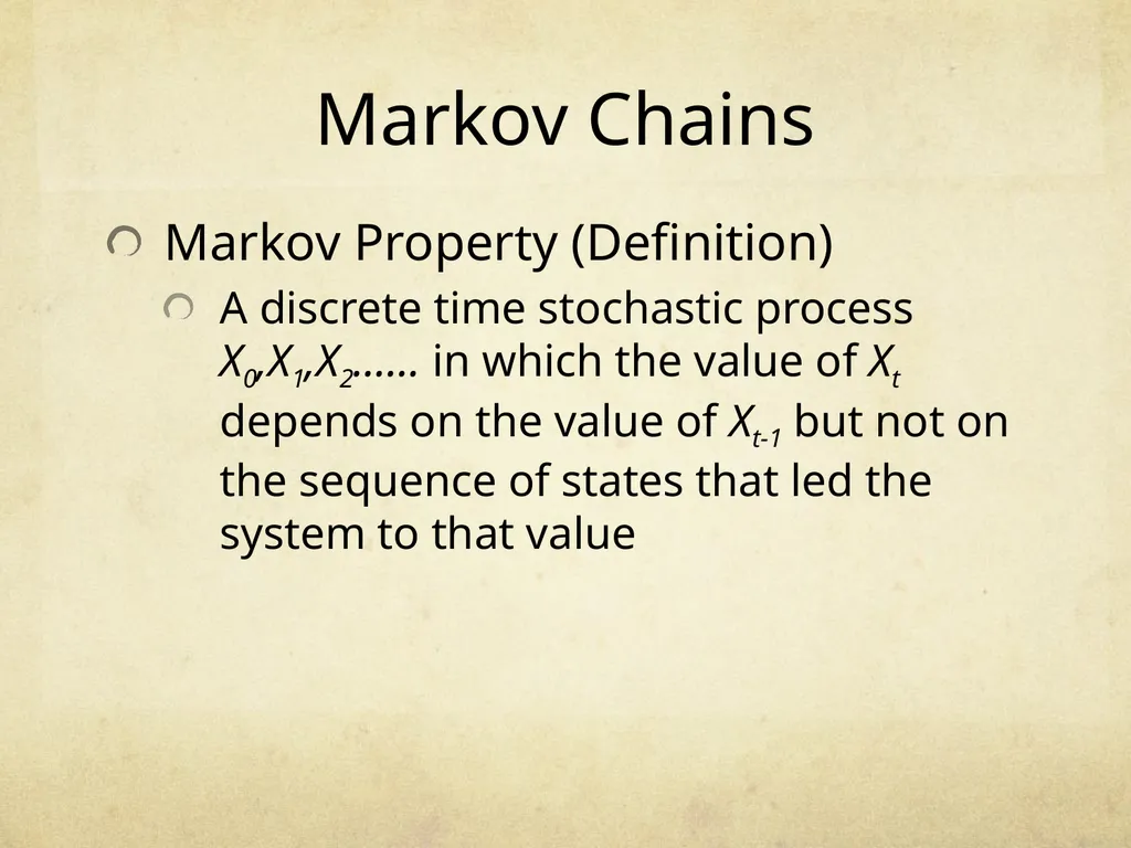
Markov Chains Markov Property (Definition)
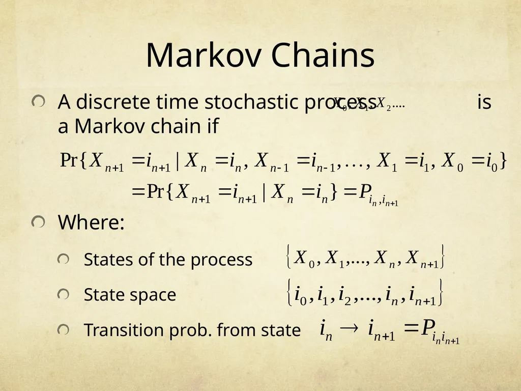
A discrete time stochastic process X0,X1,X2…… in which the value of Xt depends on the value of Xt-1 but not on the sequence of states that led the system to that value<br>
A discrete time stochastic process X0,X1,X2…… in which the value of Xt depends on the value of Xt-1 but not on the sequence of states that led the system to that value<br>
22
Markov Chains A discrete time stochastic process is a Markov chain if Where:
States of the process
State space
Transition prob. from state<br>
States of the process
State space
Transition prob. from state<br>
23
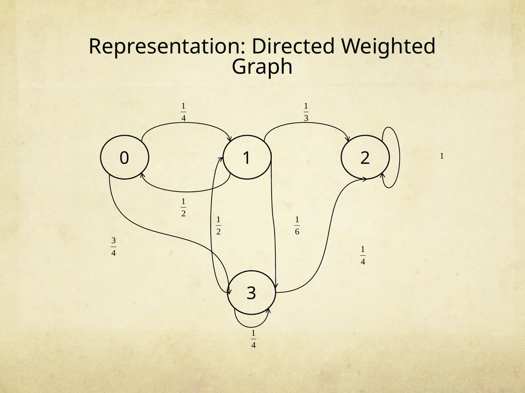
Representation: Directed Weighted Graph<br>
24
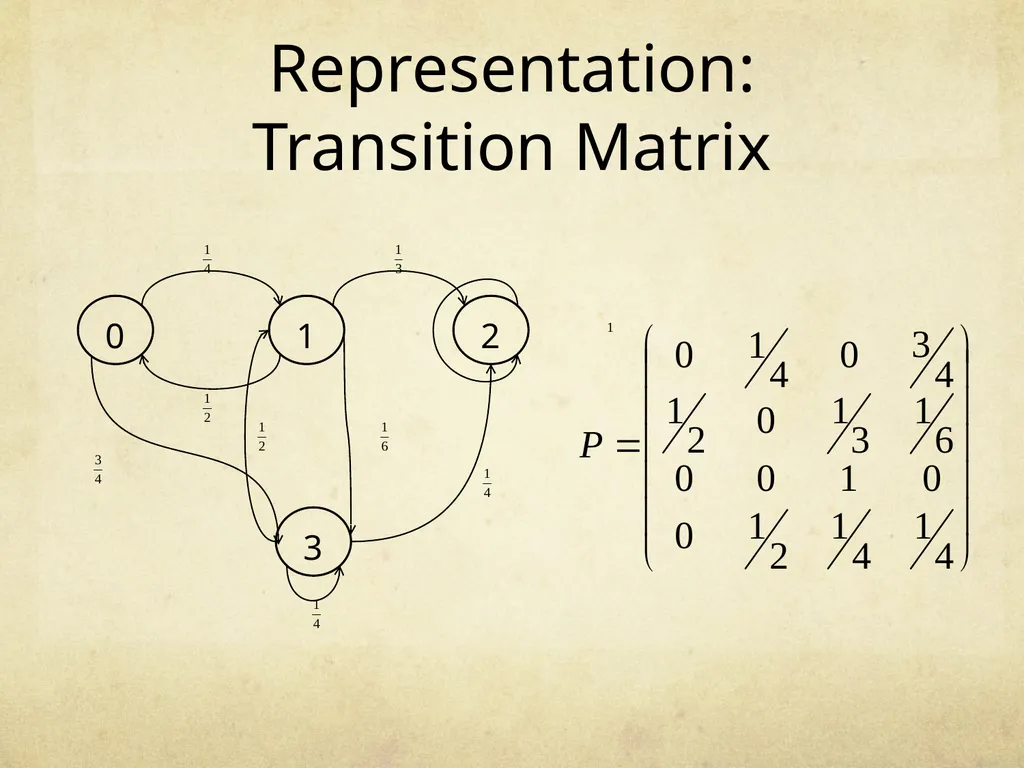
Representation: Transition Matrix<br>
25
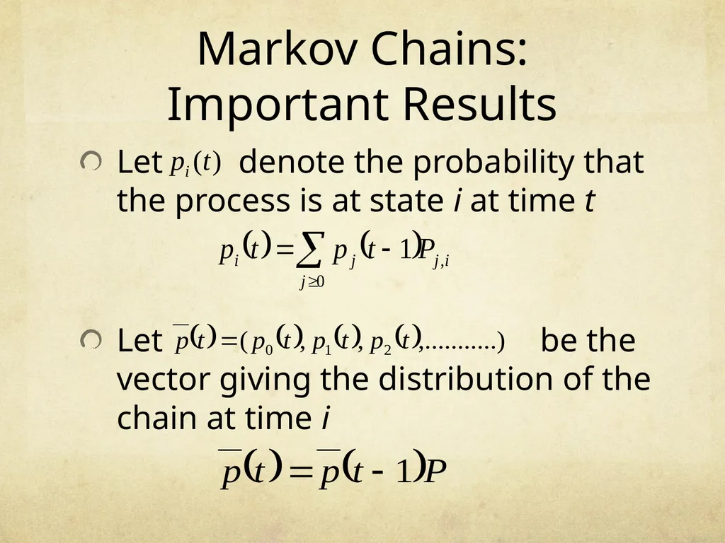
Markov Chains: Important Results Let denote the probability that the process is at state i at time t
Let be the vector giving the distribution of the chain at time i<br>
Let be the vector giving the distribution of the chain at time i<br>
26
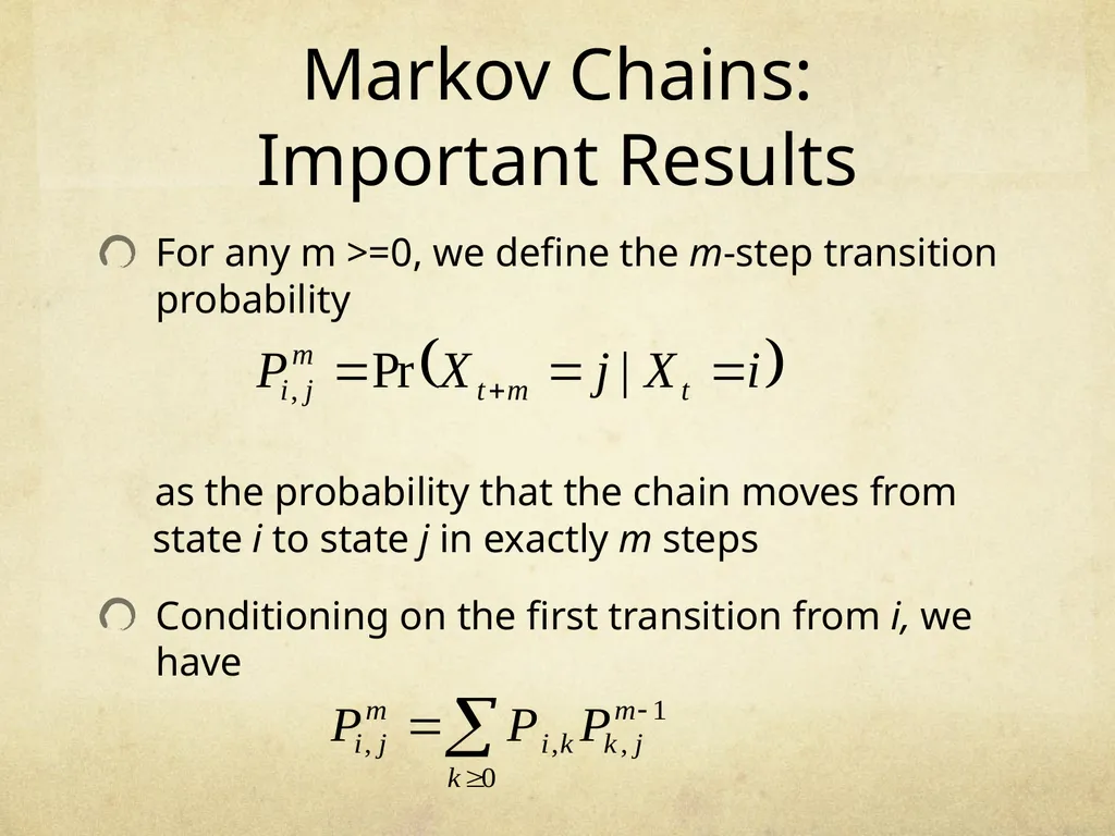
Markov Chains: Important Results For any m >=0, we define the m-step transition probability
as the probability that the chain moves from state i to state j in exactly m steps
Conditioning on the first transition from i, we have<br>
as the probability that the chain moves from state i to state j in exactly m steps
Conditioning on the first transition from i, we have<br>
27
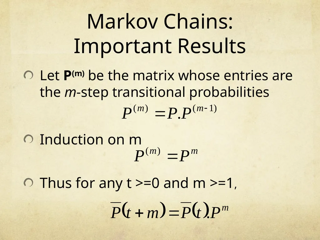
Markov Chains: Important Results Let P(m) be the matrix whose entries are the m-step transitional probabilities Induction on m Thus for any t >=0 and m >=1,<br>
28
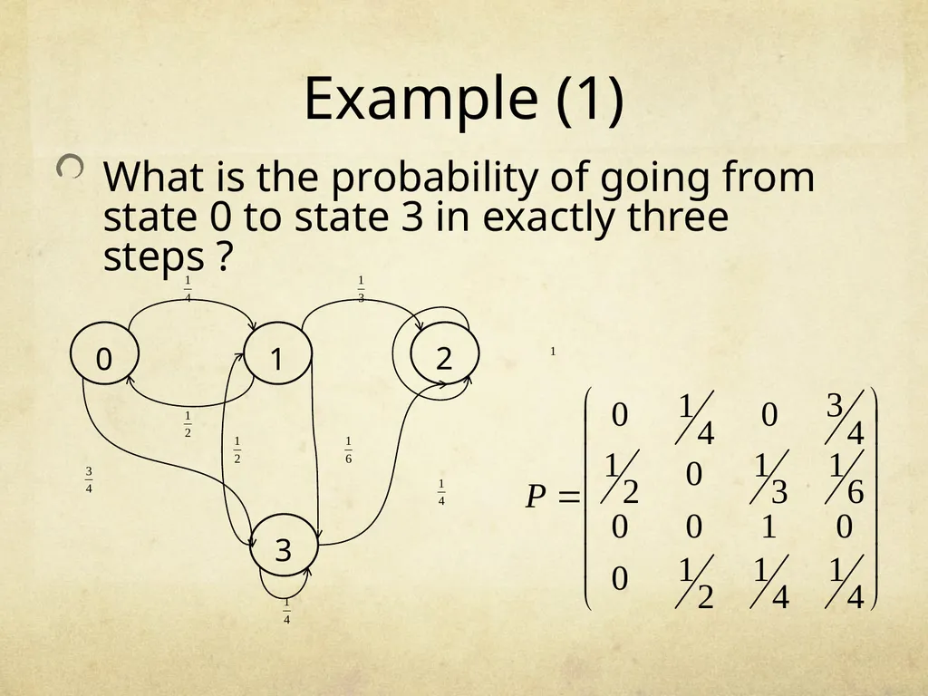
Example (1) What is the probability of going from state 0 to state 3 in exactly three steps ?<br>
29
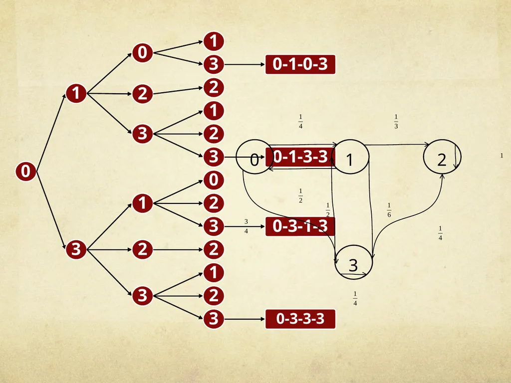
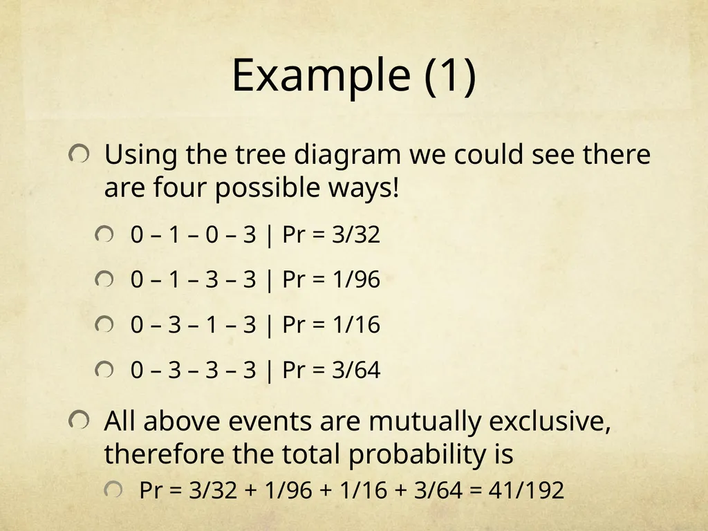
Example (1) Using the tree diagram we could see there are four possible ways!
0 – 1 – 0 – 3 | Pr = 3/32
0 – 1 – 3 – 3 | Pr = 1/96
0 – 3 – 1 – 3 | Pr = 1/16
0 – 3 – 3 – 3 | Pr = 3/64
All above events are mutually exclusive, therefore the total probability is
Pr = 3/32 + 1/96 + 1/16 + 3/64 = 41/192<br>
0 – 1 – 0 – 3 | Pr = 3/32
0 – 1 – 3 – 3 | Pr = 1/96
0 – 3 – 1 – 3 | Pr = 1/16
0 – 3 – 3 – 3 | Pr = 3/64
All above events are mutually exclusive, therefore the total probability is
Pr = 3/32 + 1/96 + 1/16 + 3/64 = 41/192<br>
30
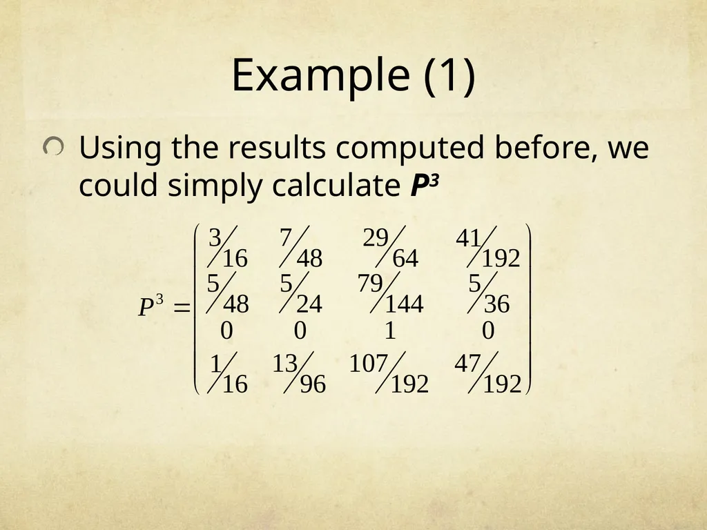
Example (1) Using the results computed before, we could simply calculate P3<br>
31
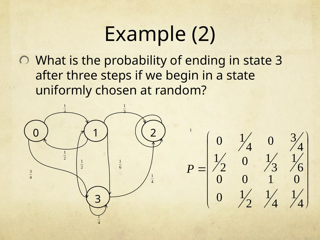
Example (2) What is the probability of ending in state 3 after three steps if we begin in a state uniformly chosen at random?<br>
32
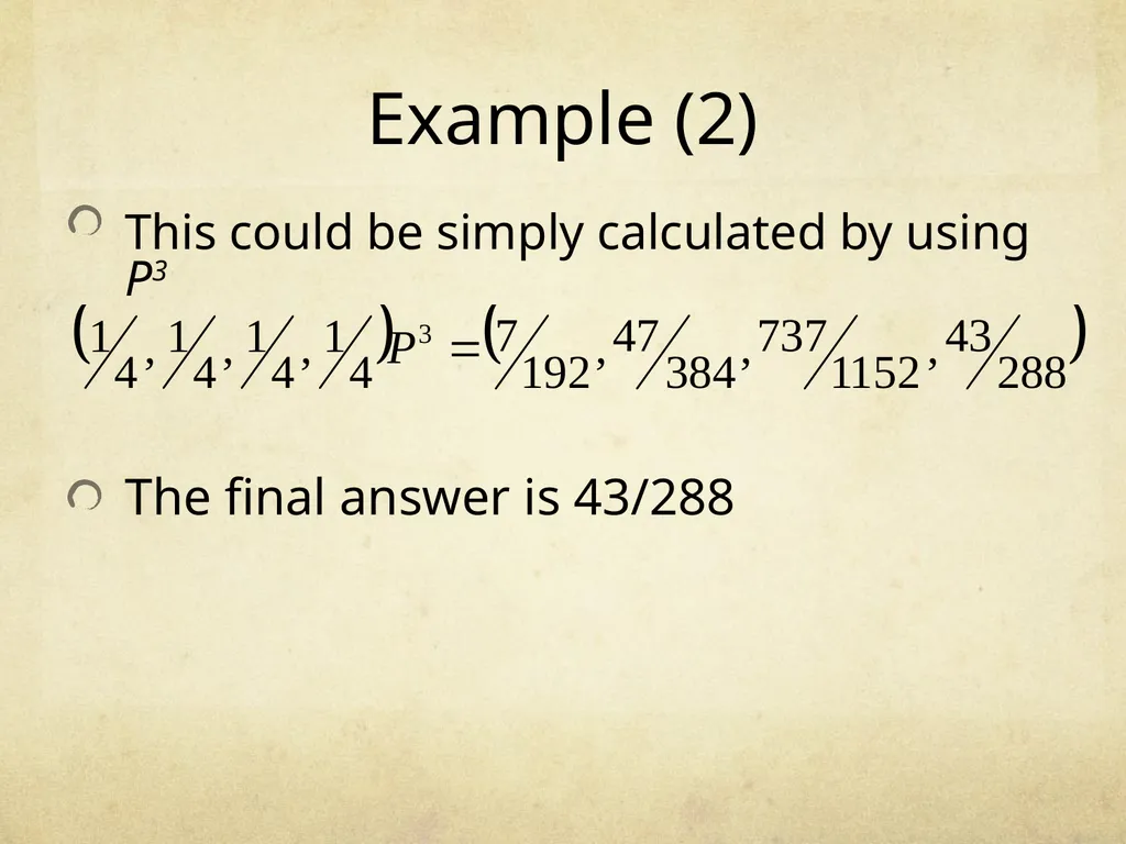
Example (2) This could be simply calculated by using P3 The final answer is 43/288<br>
33
Why do we need Markov Chains? We will be introducing three randomized algorithms
2 SAT, 3 SAT & Card Shuffling
Use of Markov Chains model the problem
Helpful in analysis of the problem<br>
2 SAT, 3 SAT & Card Shuffling
Use of Markov Chains model the problem
Helpful in analysis of the problem<br>
34
Application 1 – 2SAT<br>
35
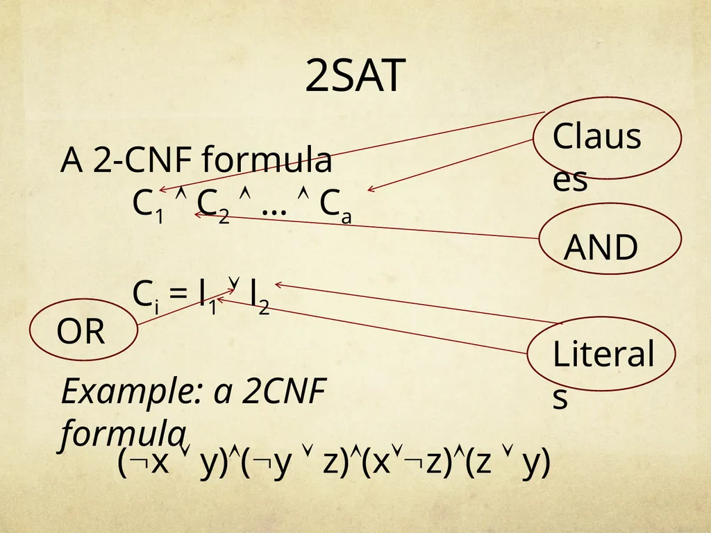
Example: a 2CNF formula (x y)(y z)(xz)(z y) Literals A 2-CNF formula
C1 C2 … Ca
Ci = l1 l2 Clauses AND OR 2SAT<br>
C1 C2 … Ca
Ci = l1 l2 Clauses AND OR 2SAT<br>
36
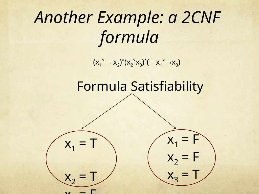
(x1 x2)(x2x3)( x1 x3) x1 = T
x2 = T
x3 = F x1 = F
x2 = F
x3 = T Formula Satisfiability Another Example: a 2CNF formula<br>
x2 = T
x3 = F x1 = F
x2 = F
x3 = T Formula Satisfiability Another Example: a 2CNF formula<br>
37
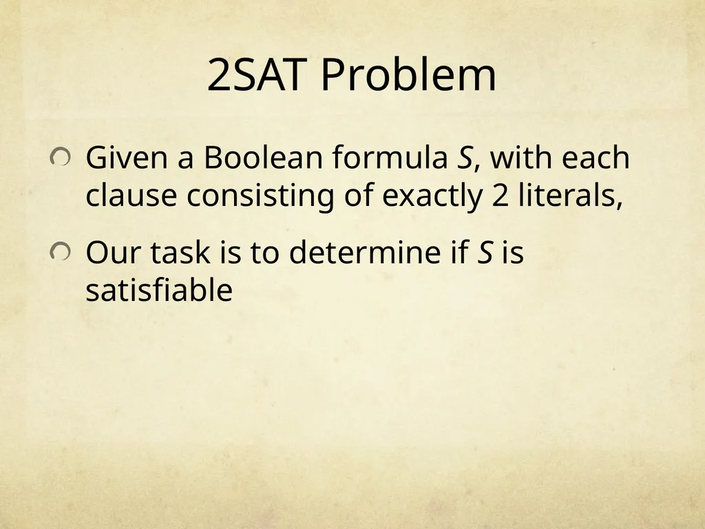
Given a Boolean formula S, with each clause consisting of exactly 2 literals,
Our task is to determine if S is satisfiable 2SAT Problem<br>
Our task is to determine if S is satisfiable 2SAT Problem<br>
38
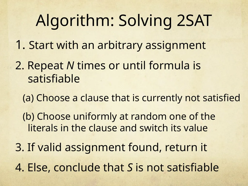
Algorithm: Solving 2SAT 1. Start with an arbitrary assignment
2. Repeat N times or until formula is satisfiable
(a) Choose a clause that is currently not satisfied
(b) Choose uniformly at random one of the literals in the clause and switch its value
3. If valid assignment found, return it
4. Else, conclude that S is not satisfiable<br>
2. Repeat N times or until formula is satisfiable
(a) Choose a clause that is currently not satisfied
(b) Choose uniformly at random one of the literals in the clause and switch its value
3. If valid assignment found, return it
4. Else, conclude that S is not satisfiable<br>
39
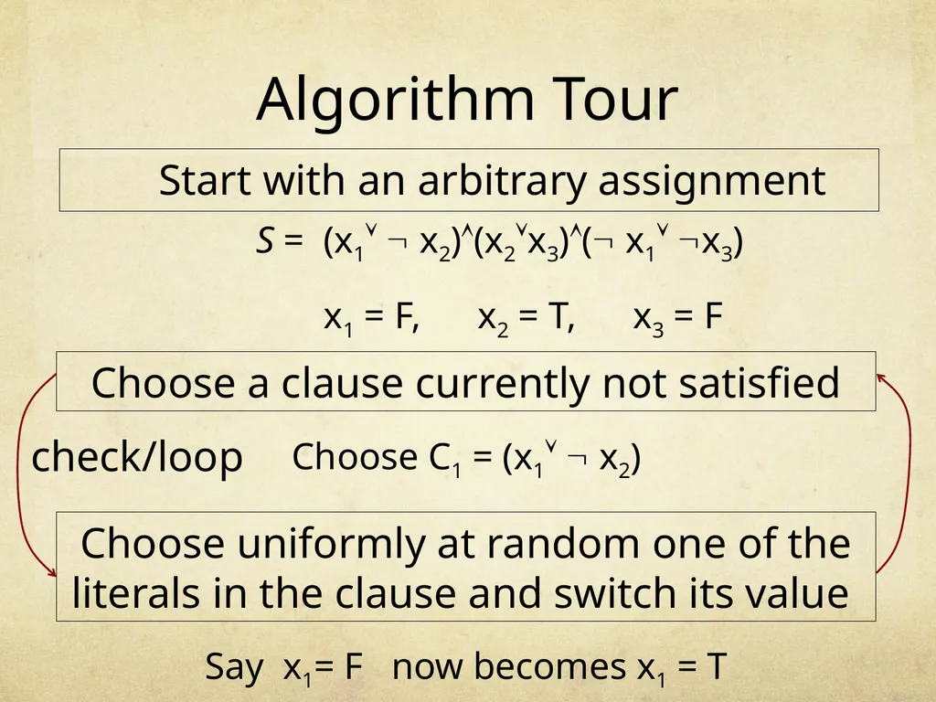
Start with an arbitrary assignment S = (x1 x2)(x2x3)( x1 x3)
x1 = F, x2 = T, x3 = F Choose a clause currently not satisfied Choose uniformly at random one of the literals in the clause and switch its value Choose C1 = (x1 x2) check/loop Say x1= F now becomes x1 = T Algorithm Tour<br>
x1 = F, x2 = T, x3 = F Choose a clause currently not satisfied Choose uniformly at random one of the literals in the clause and switch its value Choose C1 = (x1 x2) check/loop Say x1= F now becomes x1 = T Algorithm Tour<br>
40
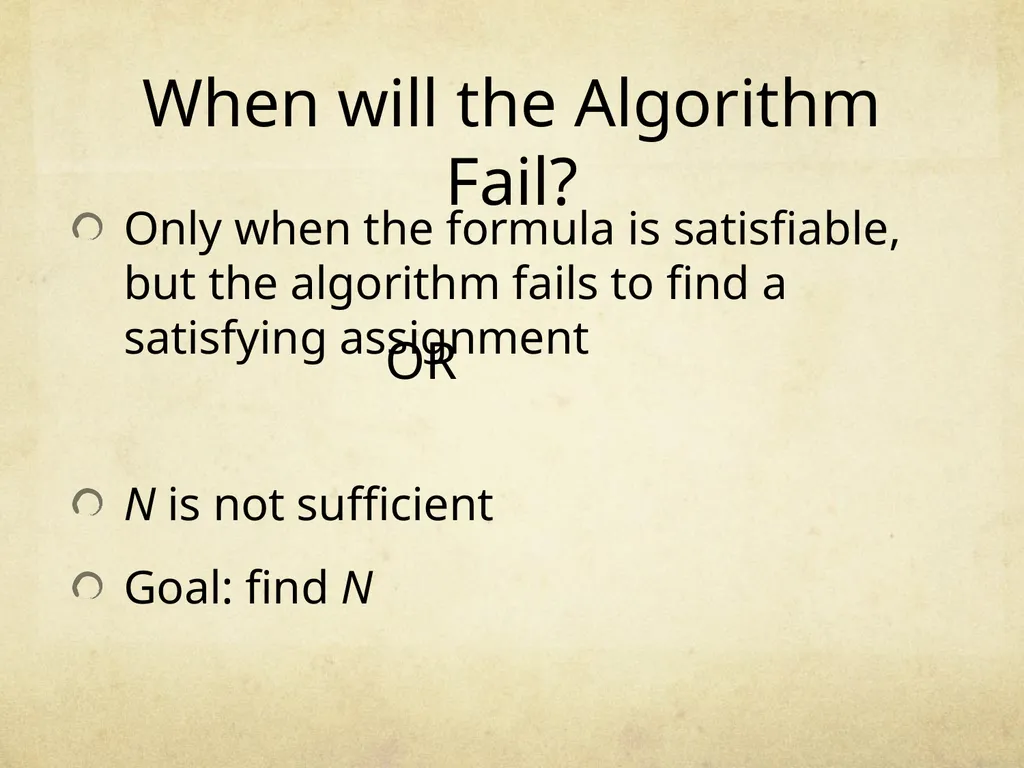
OR Only when the formula is satisfiable, but the algorithm fails to find a satisfying assignment
N is not sufficient
Goal: find N When will the Algorithm Fail?<br>
N is not sufficient
Goal: find N When will the Algorithm Fail?<br>
41
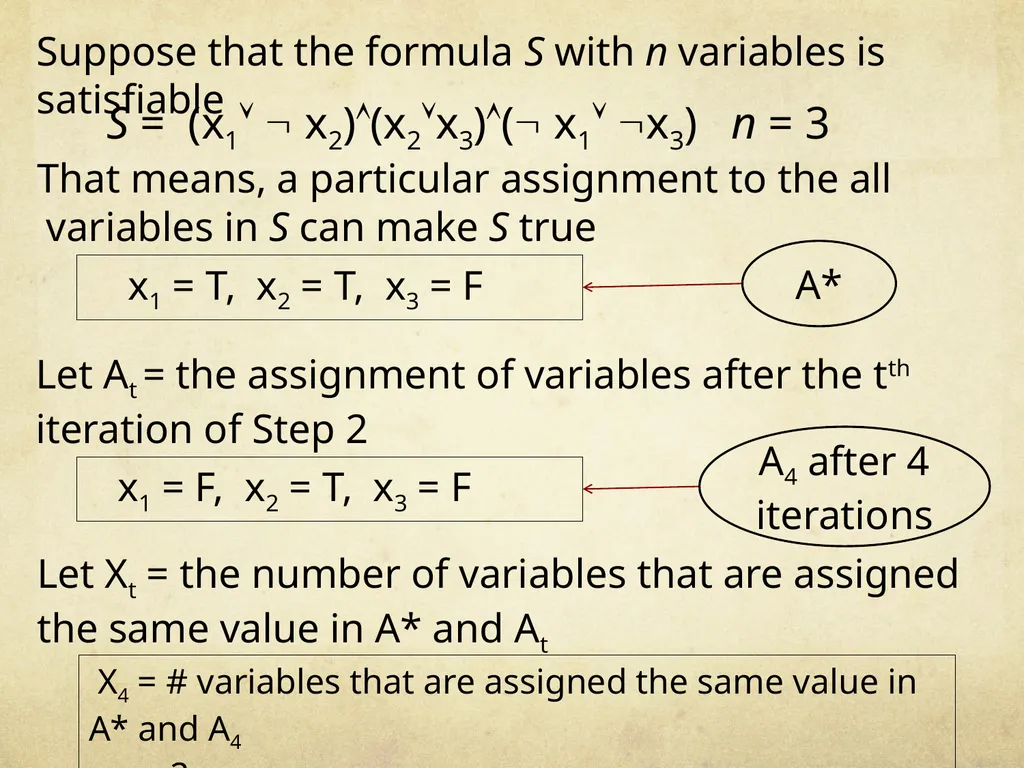
Let Xt = the number of variables that are assigned the same value in A* and At S = (x1 x2)(x2x3)( x1 x3) n = 3 Suppose that the formula S with n variables is satisfiable That means, a particular assignment to the all variables in S can make S true x1 = T, x2 = T, x3 = F A* Let At = the assignment of variables after the tth iteration of Step 2 x1 = F, x2 = T, x3 = F A4 after 4 iterations X4 = # variables that are assigned the same value in A* and A4
= 2<br>
= 2<br>
42
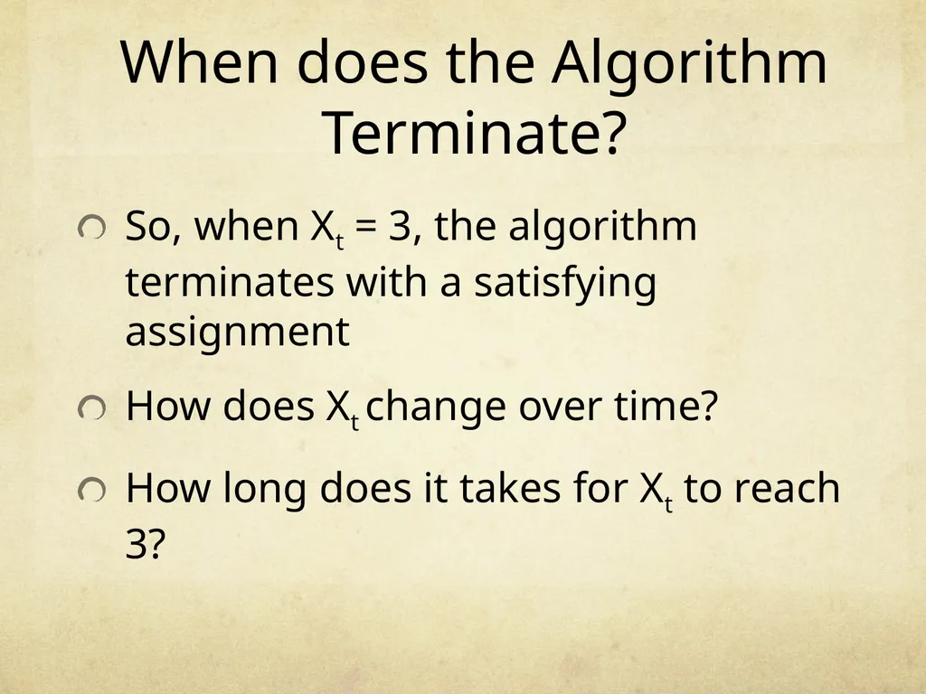
When does the Algorithm Terminate? So, when Xt = 3, the algorithm terminates with a satisfying assignment
How does Xt change over time?
How long does it takes for Xt to reach 3?<br>
How does Xt change over time?
How long does it takes for Xt to reach 3?<br>
43
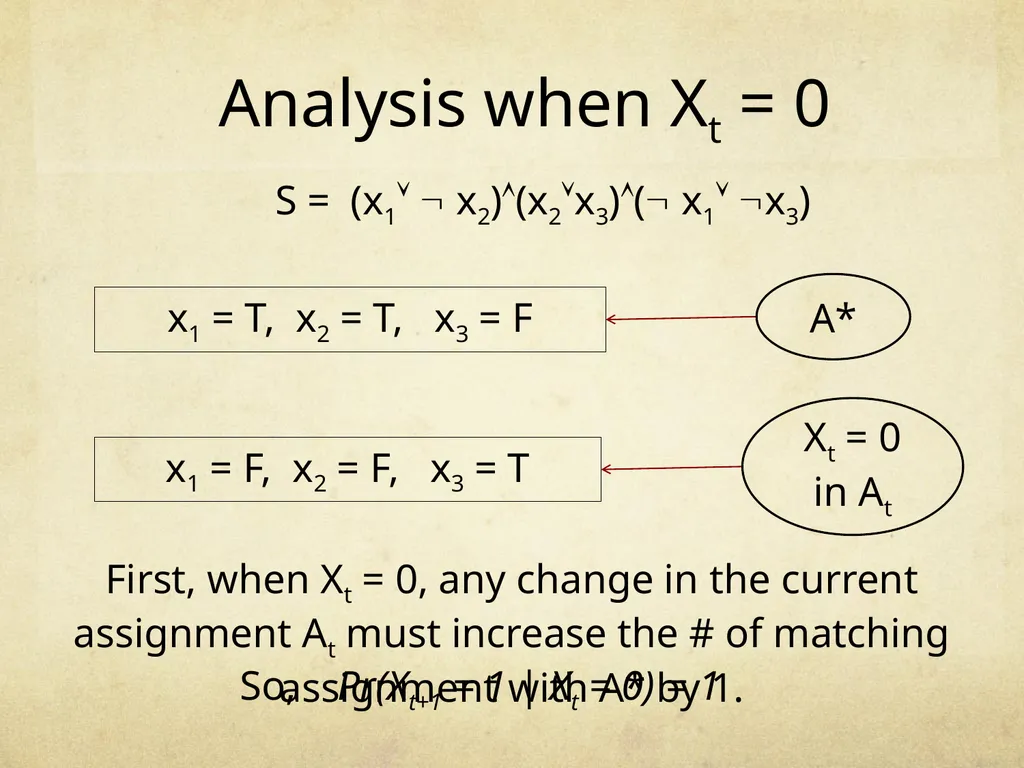
First, when Xt = 0, any change in the current assignment At must increase the # of matching assignment with A* by 1. S = (x1 x2)(x2x3)( x1 x3) x1 = T, x2 = T, x3 = F A* x1 = F, x2 = F, x3 = T Xt = 0 in At So, Pr(Xt+1 = 1 | Xt = 0) = 1 Analysis when Xt = 0<br>
44
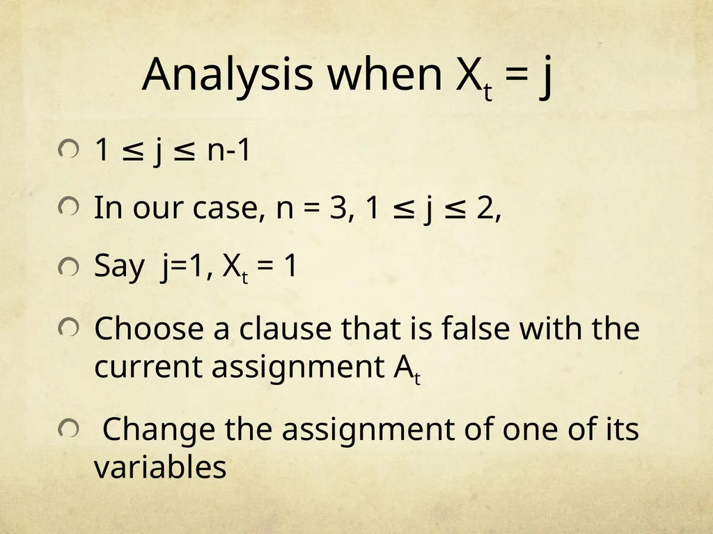
1 ≤ j ≤ n-1
In our case, n = 3, 1 ≤ j ≤ 2,
Say j=1, Xt = 1
Choose a clause that is false with the current assignment At
Change the assignment of one of its variables Analysis when Xt = j<br>
In our case, n = 3, 1 ≤ j ≤ 2,
Say j=1, Xt = 1
Choose a clause that is false with the current assignment At
Change the assignment of one of its variables Analysis when Xt = j<br>
45
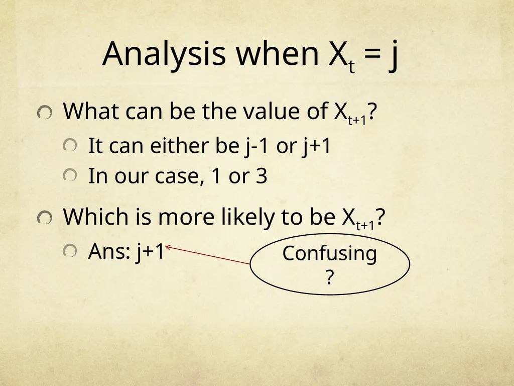
What can be the value of Xt+1?
It can either be j-1 or j+1
In our case, 1 or 3
Which is more likely to be Xt+1?
Ans: j+1 Confusing? Analysis when Xt = j<br>
It can either be j-1 or j+1
In our case, 1 or 3
Which is more likely to be Xt+1?
Ans: j+1 Confusing? Analysis when Xt = j<br>
46
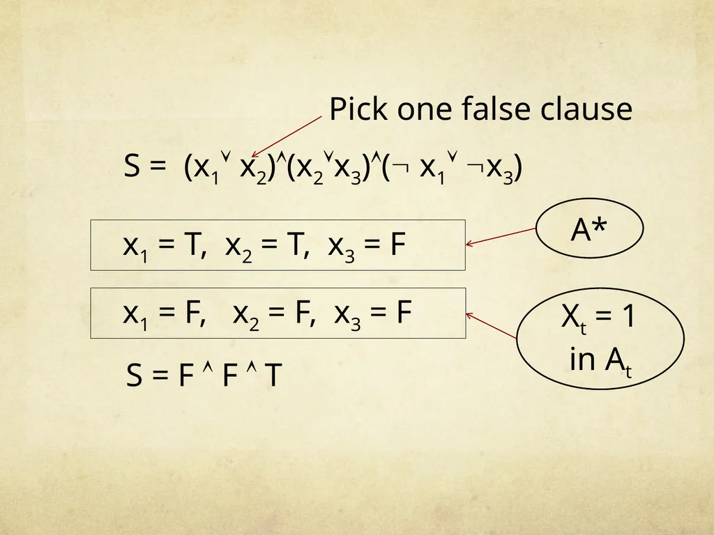
S = (x1 x2)(x2x3)( x1 x3) x1 = T, x2 = T, x3 = F A* x1 = F, x2 = F, x3 = F Xt = 1 in At Pick one false clause S = F F T<br>
47
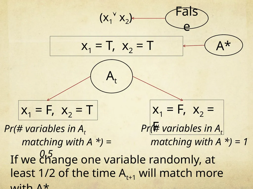
If we change one variable randomly, at least 1/2 of the time At+1 will match more with A* (x1 x2) x1 = T, x2 = T A* x1 = F, x2 = T At False x1 = F, x2 = F Pr(# variables in At
matching with A *) = 0.5 Pr(# variables in At
matching with A *) = 1<br>
matching with A *) = 0.5 Pr(# variables in At
matching with A *) = 1<br>
48
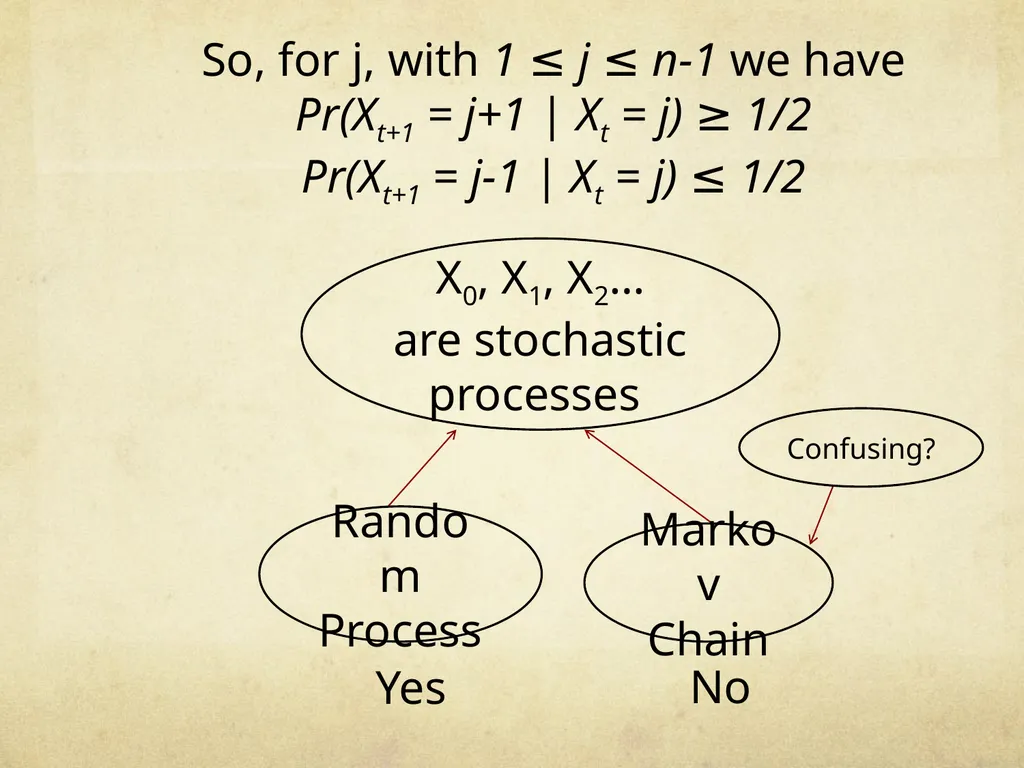
So, for j, with 1 ≤ j ≤ n-1 we have
Pr(Xt+1 = j+1 | Xt = j) ≥ 1/2
Pr(Xt+1 = j-1 | Xt = j) ≤ 1/2 X0, X1, X2…
are stochastic processes Random Process Yes Markov Chain No Confusing?<br>
Pr(Xt+1 = j+1 | Xt = j) ≥ 1/2
Pr(Xt+1 = j-1 | Xt = j) ≤ 1/2 X0, X1, X2…
are stochastic processes Random Process Yes Markov Chain No Confusing?<br>
49
Pr(Xt+1 = j+1 | Xt = j) is not a constant This value depends on which j variables are matching with A*, which in fact depends on the history of how we obtain At x1 = T, x2 = T, x3 = F A* x1 = F, x2 = F, x3 = F Xt = 1 in At x1 = F, x2 = T, x3 = T Pr(Xt+1 = 2 | Xt = 1) = 0.5 Pr(Xt+1 = 2 | Xt = 1) = 1<br>
50
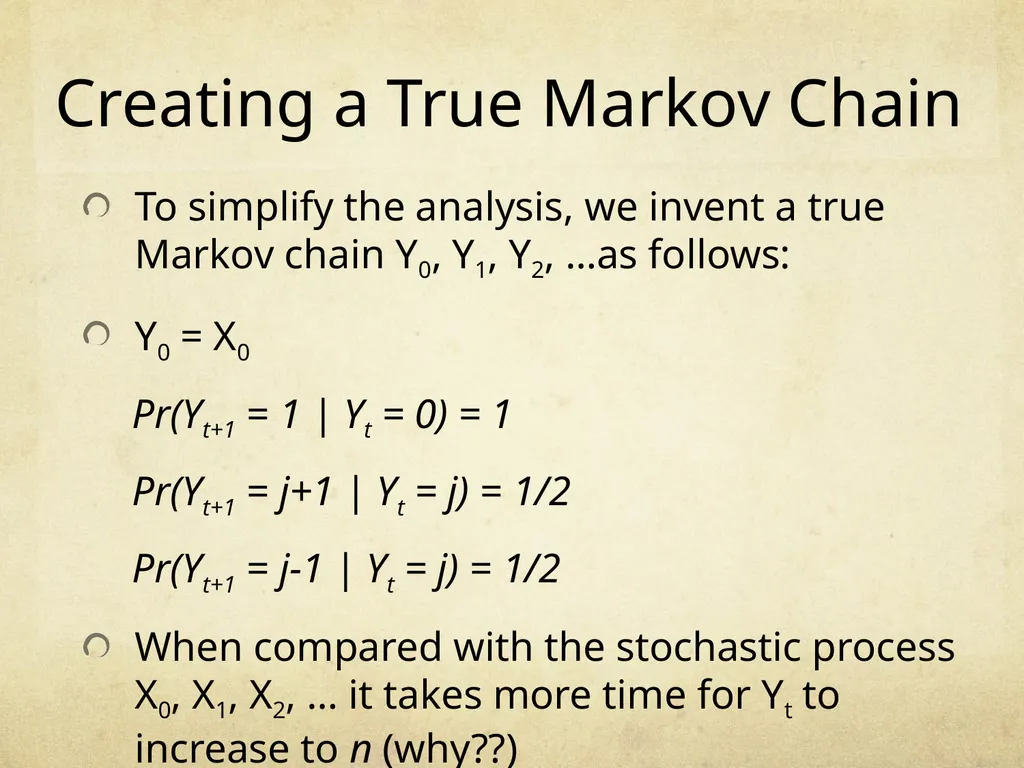
To simplify the analysis, we invent a true Markov chain Y0, Y1, Y2, …as follows:
Y0 = X0
Pr(Yt+1 = 1 | Yt = 0) = 1
Pr(Yt+1 = j+1 | Yt = j) = 1/2
Pr(Yt+1 = j-1 | Yt = j) = 1/2
When compared with the stochastic process X0, X1, X2, … it takes more time for Yt to increase to n (why??) Creating a True Markov Chain<br>
Y0 = X0
Pr(Yt+1 = 1 | Yt = 0) = 1
Pr(Yt+1 = j+1 | Yt = j) = 1/2
Pr(Yt+1 = j-1 | Yt = j) = 1/2
When compared with the stochastic process X0, X1, X2, … it takes more time for Yt to increase to n (why??) Creating a True Markov Chain<br>
51
Analysis - Time Du = Expected number of steps to reach any destination, starting from position u
Du = 1 + 0.5 Du-1 + 0.5 Du+1
Dv = 1 + 0.5 Dv-1 + Dv+1<br>
Du = 1 + 0.5 Du-1 + 0.5 Du+1
Dv = 1 + 0.5 Dv-1 + Dv+1<br>
52
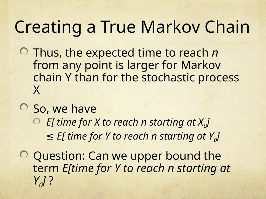
Thus, the expected time to reach n from any point is larger for Markov chain Y than for the stochastic process X
So, we have
E[ time for X to reach n starting at X0]
≤ E[ time for Y to reach n starting at Y0]
Question: Can we upper bound the term E[time for Y to reach n starting at Y0] ? Creating a True Markov Chain<br>
So, we have
E[ time for X to reach n starting at X0]
≤ E[ time for Y to reach n starting at Y0]
Question: Can we upper bound the term E[time for Y to reach n starting at Y0] ? Creating a True Markov Chain<br>
53
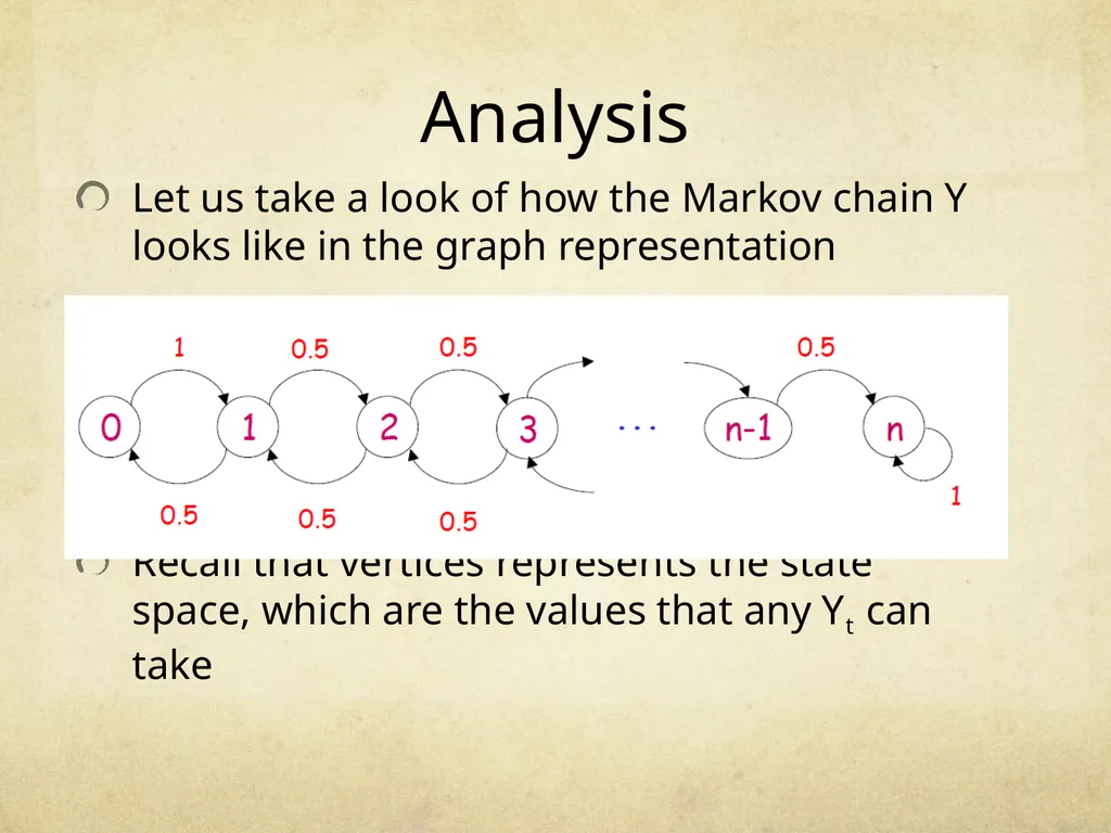
Analysis Let us take a look of how the Markov chain Y looks like in the graph representation
Recall that vertices represents the state space, which are the values that any Yt can take<br>
Recall that vertices represents the state space, which are the values that any Yt can take<br>
54
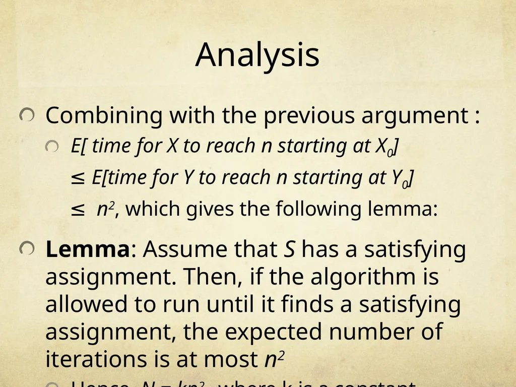
Analysis Combining with the previous argument :
E[ time for X to reach n starting at X0]
≤ E[time for Y to reach n starting at Y0]
≤ n2, which gives the following lemma:
Lemma: Assume that S has a satisfying assignment. Then, if the algorithm is allowed to run until it finds a satisfying assignment, the expected number of iterations is at most n2
Hence, N = kn2 , where k is a constant<br>
E[ time for X to reach n starting at X0]
≤ E[time for Y to reach n starting at Y0]
≤ n2, which gives the following lemma:
Lemma: Assume that S has a satisfying assignment. Then, if the algorithm is allowed to run until it finds a satisfying assignment, the expected number of iterations is at most n2
Hence, N = kn2 , where k is a constant<br>
55
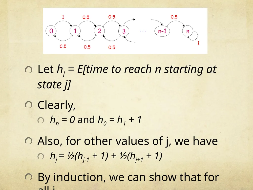
Let hj = E[time to reach n starting at state j]
Clearly,
hn = 0 and h0 = h1 + 1
Also, for other values of j, we have
hj = ½(hj-1 + 1) + ½(hj+1 + 1)
By induction, we can show that for all j,
hj = n2 –j2 ≤ n2<br>
Clearly,
hn = 0 and h0 = h1 + 1
Also, for other values of j, we have
hj = ½(hj-1 + 1) + ½(hj+1 + 1)
By induction, we can show that for all j,
hj = n2 –j2 ≤ n2<br>
56
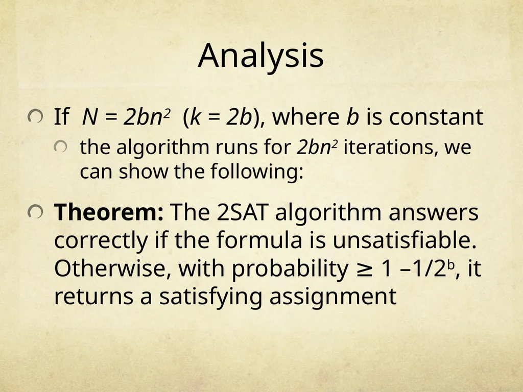
Analysis If N = 2bn2 (k = 2b), where b is constant
the algorithm runs for 2bn2 iterations, we can show the following:
Theorem: The 2SAT algorithm answers correctly if the formula is unsatisfiable. Otherwise, with probability ≥ 1 –1/2b, it returns a satisfying assignment<br>
the algorithm runs for 2bn2 iterations, we can show the following:
Theorem: The 2SAT algorithm answers correctly if the formula is unsatisfiable. Otherwise, with probability ≥ 1 –1/2b, it returns a satisfying assignment<br>
57
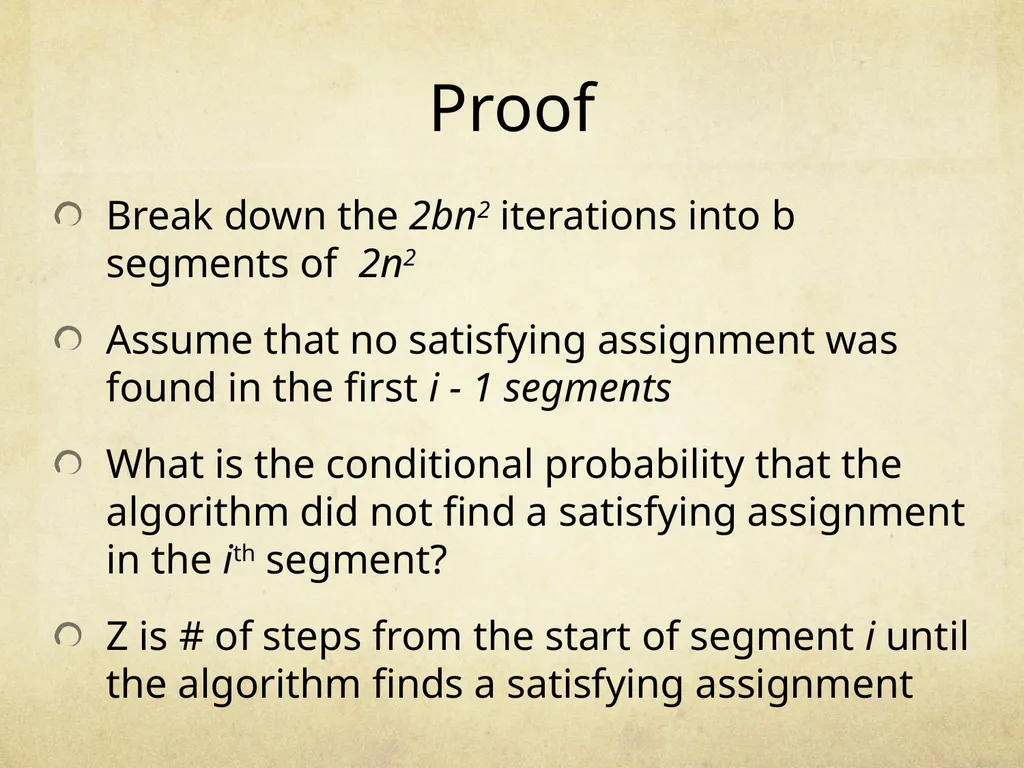
Break down the 2bn2 iterations into b segments of 2n2
Assume that no satisfying assignment was found in the first i - 1 segments
What is the conditional probability that the algorithm did not find a satisfying assignment in the ith segment?
Z is # of steps from the start of segment i until the algorithm finds a satisfying assignment Proof<br>
Assume that no satisfying assignment was found in the first i - 1 segments
What is the conditional probability that the algorithm did not find a satisfying assignment in the ith segment?
Z is # of steps from the start of segment i until the algorithm finds a satisfying assignment Proof<br>
58
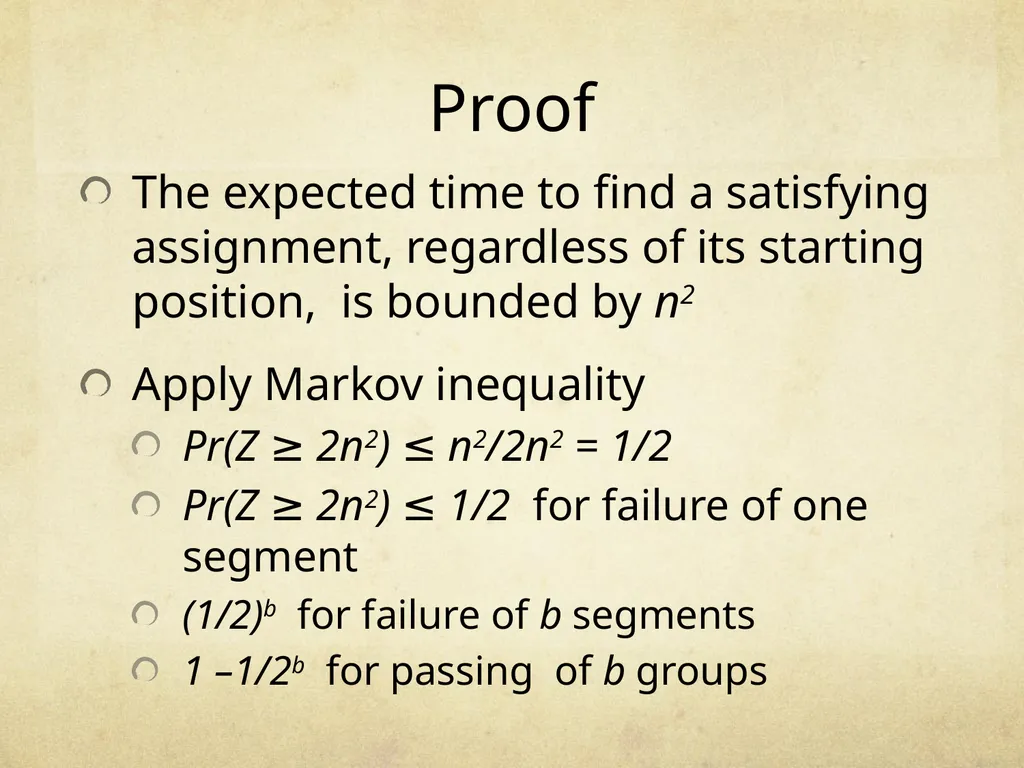
Proof The expected time to find a satisfying assignment, regardless of its starting position, is bounded by n2
Apply Markov inequality
Pr(Z ≥ 2n2) ≤ n2/2n2 = 1/2
Pr(Z ≥ 2n2) ≤ 1/2 for failure of one segment
(1/2)b for failure of b segments
1 –1/2b for passing of b groups<br>
Apply Markov inequality
Pr(Z ≥ 2n2) ≤ n2/2n2 = 1/2
Pr(Z ≥ 2n2) ≤ 1/2 for failure of one segment
(1/2)b for failure of b segments
1 –1/2b for passing of b groups<br>
59
Application 2 – 3SAT<br>
60
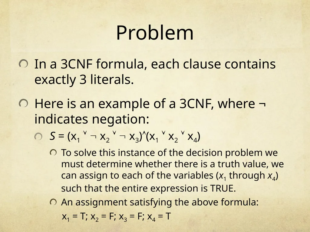
Problem In a 3CNF formula, each clause contains exactly 3 literals.
Here is an example of a 3CNF, where ¬ indicates negation:
S = (x1 x2 x3)(x1 x2 x4)
To solve this instance of the decision problem we must determine whether there is a truth value, we can assign to each of the variables (x1 through x4) such that the entire expression is TRUE.
An assignment satisfying the above formula:
x1 = T; x2 = F; x3 = F; x4 = T<br>
Here is an example of a 3CNF, where ¬ indicates negation:
S = (x1 x2 x3)(x1 x2 x4)
To solve this instance of the decision problem we must determine whether there is a truth value, we can assign to each of the variables (x1 through x4) such that the entire expression is TRUE.
An assignment satisfying the above formula:
x1 = T; x2 = F; x3 = F; x4 = T<br>
61
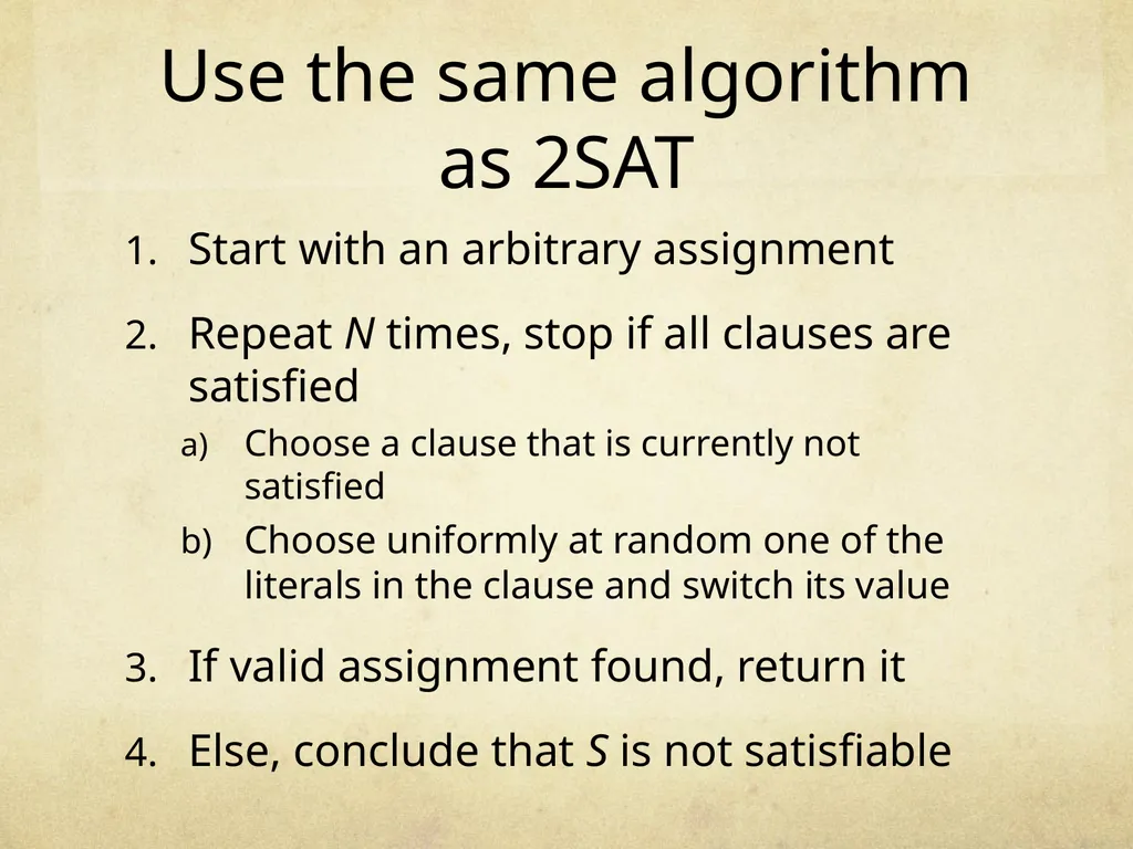
Use the same algorithm as 2SAT Start with an arbitrary assignment
Repeat N times, stop if all clauses are satisfied
Choose a clause that is currently not satisfied
Choose uniformly at random one of the literals in the clause and switch its value
If valid assignment found, return it
Else, conclude that S is not satisfiable<br>
Repeat N times, stop if all clauses are satisfied
Choose a clause that is currently not satisfied
Choose uniformly at random one of the literals in the clause and switch its value
If valid assignment found, return it
Else, conclude that S is not satisfiable<br>
62
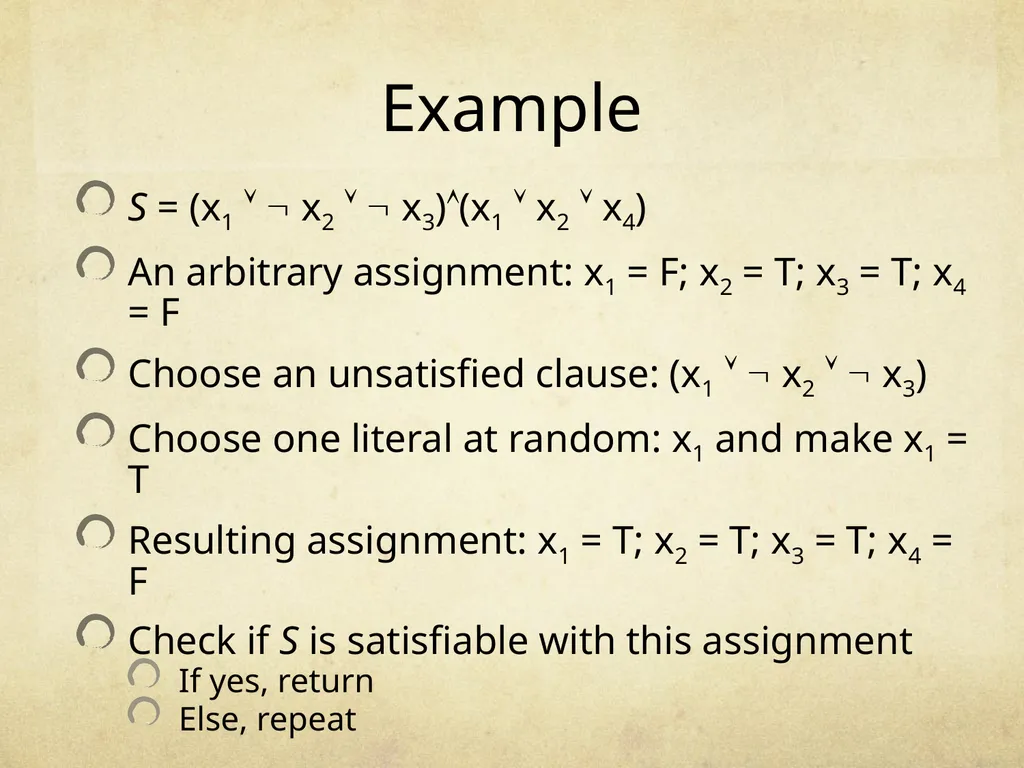
Example S = (x1 x2 x3)(x1 x2 x4)
An arbitrary assignment: x1 = F; x2 = T; x3 = T; x4 = F
Choose an unsatisfied clause: (x1 x2 x3)
Choose one literal at random: x1 and make x1 = T
Resulting assignment: x1 = T; x2 = T; x3 = T; x4 = F
Check if S is satisfiable with this assignment
If yes, return
Else, repeat<br>
An arbitrary assignment: x1 = F; x2 = T; x3 = T; x4 = F
Choose an unsatisfied clause: (x1 x2 x3)
Choose one literal at random: x1 and make x1 = T
Resulting assignment: x1 = T; x2 = T; x3 = T; x4 = F
Check if S is satisfiable with this assignment
If yes, return
Else, repeat<br>
63
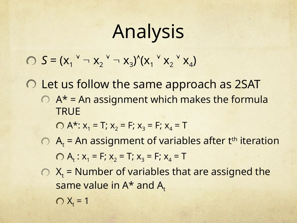
Analysis S = (x1 x2 x3)(x1 x2 x4)
Let us follow the same approach as 2SAT
A* = An assignment which makes the formula TRUE
A*: x1 = T; x2 = F; x3 = F; x4 = T
At = An assignment of variables after tth iteration
At : x1 = F; x2 = T; x3 = F; x4 = T
Xt = Number of variables that are assigned the same value in A* and At
Xt = 1<br>
Let us follow the same approach as 2SAT
A* = An assignment which makes the formula TRUE
A*: x1 = T; x2 = F; x3 = F; x4 = T
At = An assignment of variables after tth iteration
At : x1 = F; x2 = T; x3 = F; x4 = T
Xt = Number of variables that are assigned the same value in A* and At
Xt = 1<br>
64
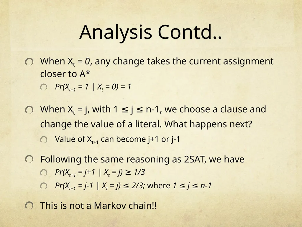
Analysis Contd.. When Xt = 0, any change takes the current assignment closer to A*
Pr(Xt+1 = 1 | Xt = 0) = 1
When Xt = j, with 1 ≤ j ≤ n-1, we choose a clause and change the value of a literal. What happens next?
Value of Xt+1 can become j+1 or j-1
Following the same reasoning as 2SAT, we have
Pr(Xt+1 = j+1 | Xt = j) ≥ 1/3
Pr(Xt+1 = j-1 | Xt = j) ≤ 2/3; where 1 ≤ j ≤ n-1
This is not a Markov chain!!<br>
Pr(Xt+1 = 1 | Xt = 0) = 1
When Xt = j, with 1 ≤ j ≤ n-1, we choose a clause and change the value of a literal. What happens next?
Value of Xt+1 can become j+1 or j-1
Following the same reasoning as 2SAT, we have
Pr(Xt+1 = j+1 | Xt = j) ≥ 1/3
Pr(Xt+1 = j-1 | Xt = j) ≤ 2/3; where 1 ≤ j ≤ n-1
This is not a Markov chain!!<br>
65
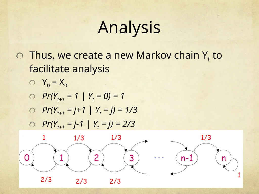
Analysis Thus, we create a new Markov chain Yt to facilitate analysis
Y0 = X0
Pr(Yt+1 = 1 | Yt = 0) = 1
Pr(Yt+1 = j+1 | Yt = j) = 1/3
Pr(Yt+1 = j-1 | Yt = j) = 2/3<br>
Y0 = X0
Pr(Yt+1 = 1 | Yt = 0) = 1
Pr(Yt+1 = j+1 | Yt = j) = 1/3
Pr(Yt+1 = j-1 | Yt = j) = 2/3<br>
66
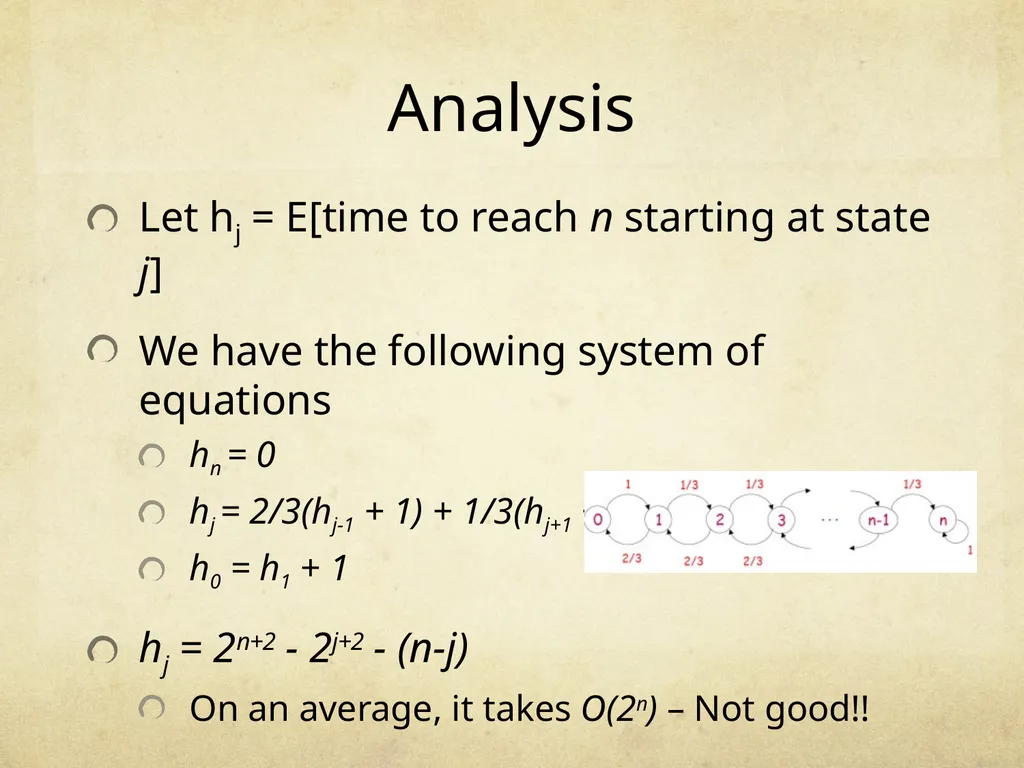
Analysis Let hj = E[time to reach n starting at state j]
We have the following system of equations
hn = 0
hj = 2/3(hj-1 + 1) + 1/3(hj+1 + 1)
h0 = h1 + 1
hj = 2n+2 - 2j+2 - (n-j)
On an average, it takes O(2n) – Not good!!<br>
We have the following system of equations
hn = 0
hj = 2/3(hj-1 + 1) + 1/3(hj+1 + 1)
h0 = h1 + 1
hj = 2n+2 - 2j+2 - (n-j)
On an average, it takes O(2n) – Not good!!<br>
67
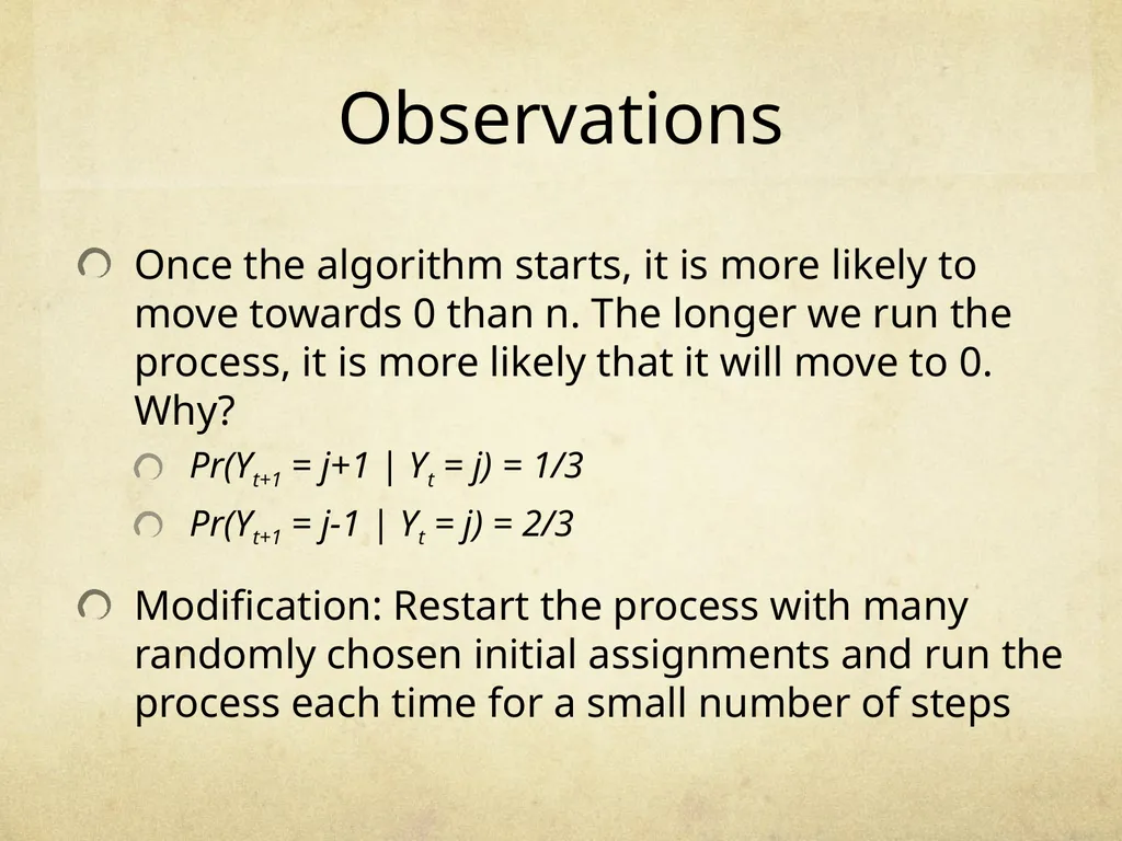
Observations Once the algorithm starts, it is more likely to move towards 0 than n. The longer we run the process, it is more likely that it will move to 0. Why?
Pr(Yt+1 = j+1 | Yt = j) = 1/3
Pr(Yt+1 = j-1 | Yt = j) = 2/3
Modification: Restart the process with many randomly chosen initial assignments and run the process each time for a small number of steps<br>
Pr(Yt+1 = j+1 | Yt = j) = 1/3
Pr(Yt+1 = j-1 | Yt = j) = 2/3
Modification: Restart the process with many randomly chosen initial assignments and run the process each time for a small number of steps<br>
68
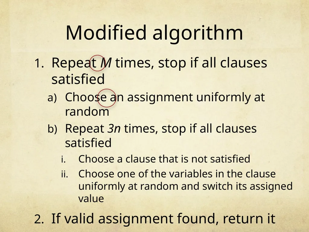
Modified algorithm Repeat M times, stop if all clauses satisfied
Choose an assignment uniformly at random
Repeat 3n times, stop if all clauses satisfied
Choose a clause that is not satisfied
Choose one of the variables in the clause uniformly at random and switch its assigned value
If valid assignment found, return it
Else, conclude that S is unsatisfiable<br>
Choose an assignment uniformly at random
Repeat 3n times, stop if all clauses satisfied
Choose a clause that is not satisfied
Choose one of the variables in the clause uniformly at random and switch its assigned value
If valid assignment found, return it
Else, conclude that S is unsatisfiable<br>
69
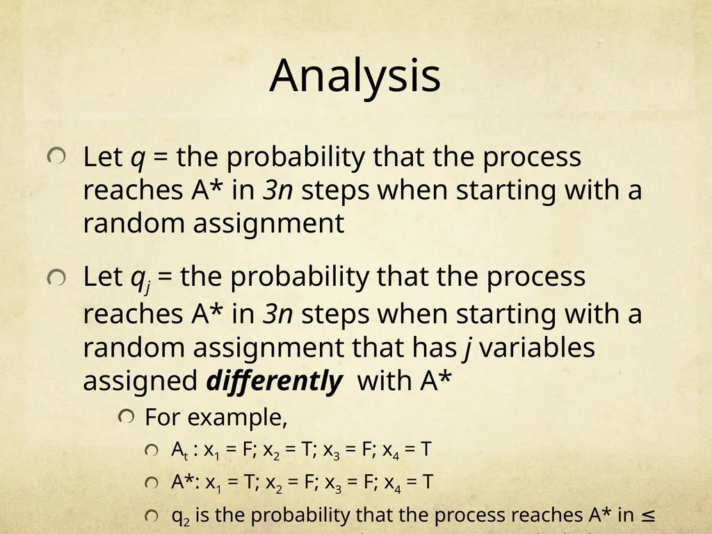
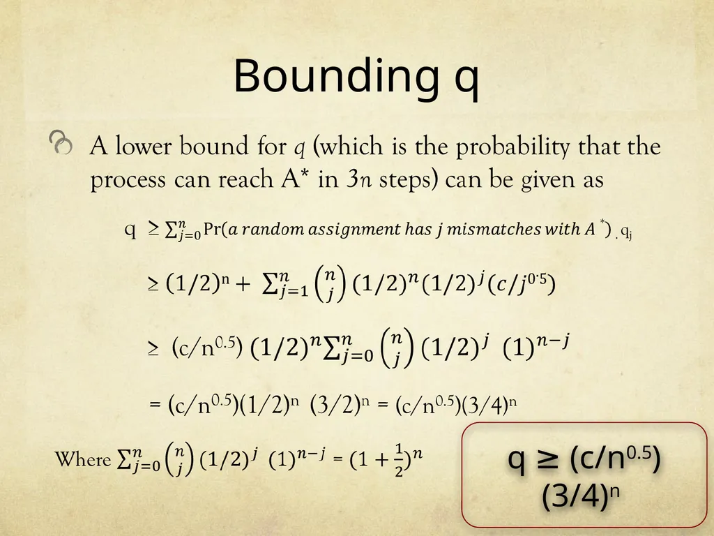
Analysis Let q = the probability that the process reaches A* in 3n steps when starting with a random assignment
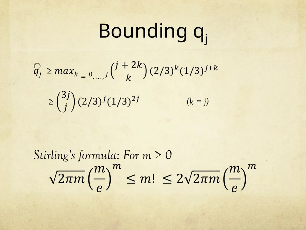
Let qj = the probability that the process reaches A* in 3n steps when starting with a random assignment that has j variables assigned differently with A*
For example,
At : x1 = F; x2 = T; x3 = F; x4 = T
A*: x1 = T; x2 = F; x3 = F; x4 = T
q2 is the probability that the process reaches A* in ≤ 3n steps starting with an assignment which disagrees with A* in 2 variables.<br>
Let qj = the probability that the process reaches A* in 3n steps when starting with a random assignment that has j variables assigned differently with A*
For example,
At : x1 = F; x2 = T; x3 = F; x4 = T
A*: x1 = T; x2 = F; x3 = F; x4 = T
q2 is the probability that the process reaches A* in ≤ 3n steps starting with an assignment which disagrees with A* in 2 variables.<br>
70
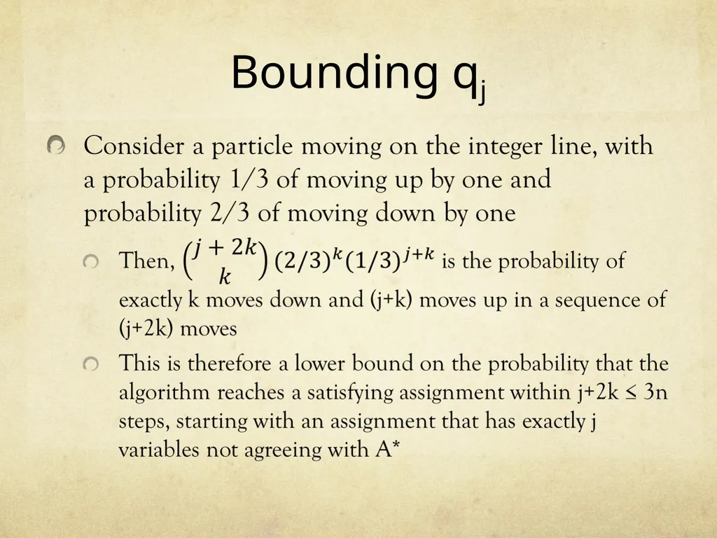
Bounding qj<br>
71
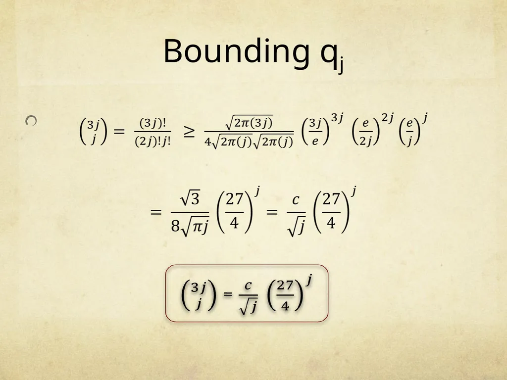
Bounding qj<br>
72
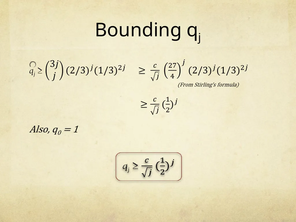
Bounding qj<br>
73
Bounding qj<br>
74
Bounding q q ≥ (c/n0.5)(3/4)n<br>
75
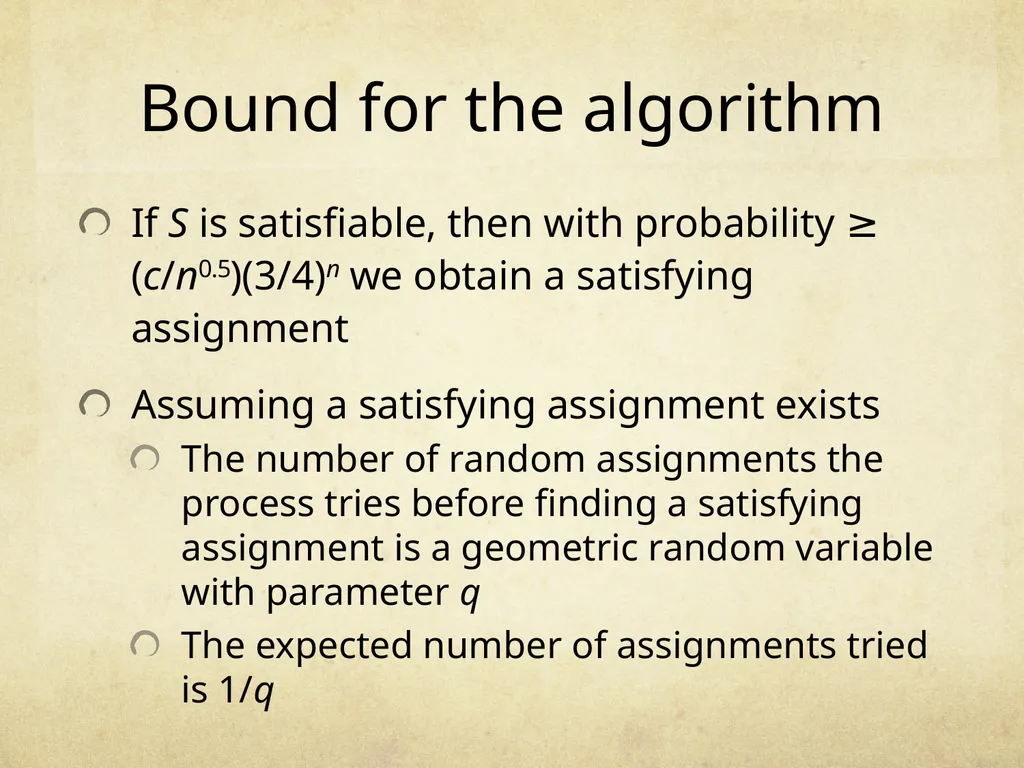
Bound for the algorithm If S is satisfiable, then with probability ≥ (c/n0.5)(3/4)n we obtain a satisfying assignment
Assuming a satisfying assignment exists
The number of random assignments the process tries before finding a satisfying assignment is a geometric random variable with parameter q
The expected number of assignments tried is 1/q<br>
Assuming a satisfying assignment exists
The number of random assignments the process tries before finding a satisfying assignment is a geometric random variable with parameter q
The expected number of assignments tried is 1/q<br>
76
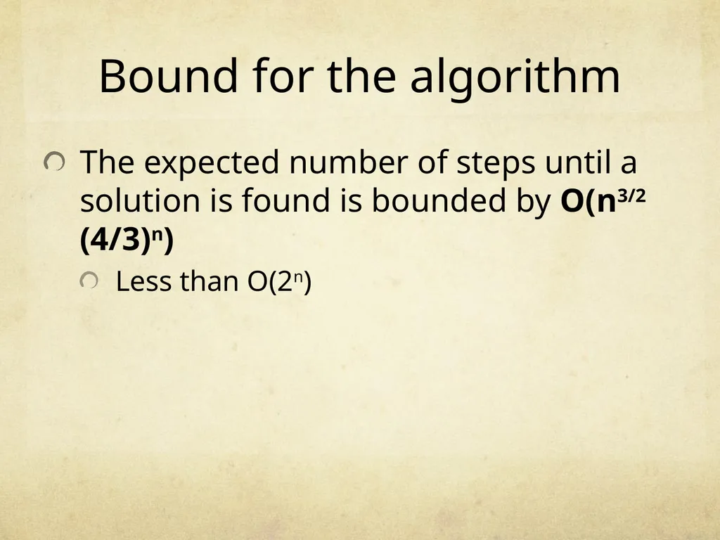
Bound for the algorithm The expected number of steps until a solution is found is bounded by O(n3/2 (4/3)n)
Less than O(2n)<br>
Less than O(2n)<br>
77
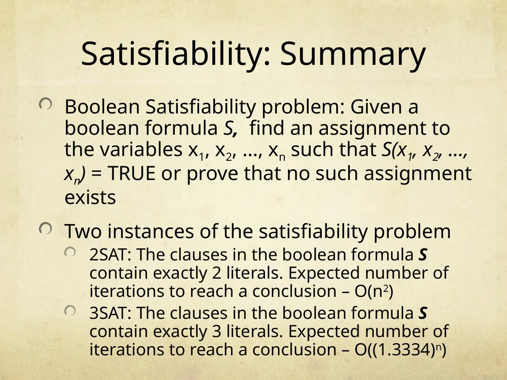
Satisfiability: Summary Boolean Satisfiability problem: Given a boolean formula S, find an assignment to the variables x1, x2, …, xn such that S(x1, x2, …, xn) = TRUE or prove that no such assignment exists
Two instances of the satisfiability problem
2SAT: The clauses in the boolean formula S contain exactly 2 literals. Expected number of iterations to reach a conclusion – O(n2)
3SAT: The clauses in the boolean formula S contain exactly 3 literals. Expected number of iterations to reach a conclusion – O((1.3334)n)<br>
Two instances of the satisfiability problem
2SAT: The clauses in the boolean formula S contain exactly 2 literals. Expected number of iterations to reach a conclusion – O(n2)
3SAT: The clauses in the boolean formula S contain exactly 3 literals. Expected number of iterations to reach a conclusion – O((1.3334)n)<br>
78
Application 3 – Card Shuffling<br>
79
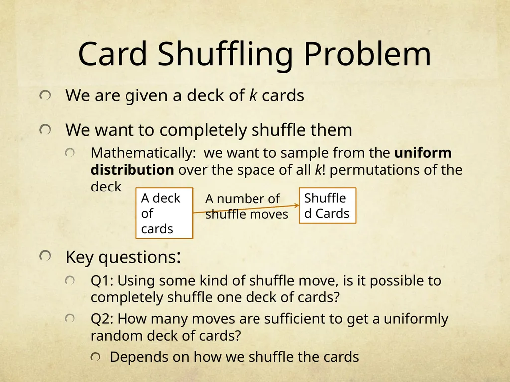
Card Shuffling Problem We are given a deck of k cards
We want to completely shuffle them
Mathematically: we want to sample from the uniform distribution over the space of all k! permutations of the deck
Key questions:
Q1: Using some kind of shuffle move, is it possible to completely shuffle one deck of cards?
Q2: How many moves are sufficient to get a uniformly random deck of cards?
Depends on how we shuffle the cards<br>
We want to completely shuffle them
Mathematically: we want to sample from the uniform distribution over the space of all k! permutations of the deck
Key questions:
Q1: Using some kind of shuffle move, is it possible to completely shuffle one deck of cards?
Q2: How many moves are sufficient to get a uniformly random deck of cards?
Depends on how we shuffle the cards<br>
80
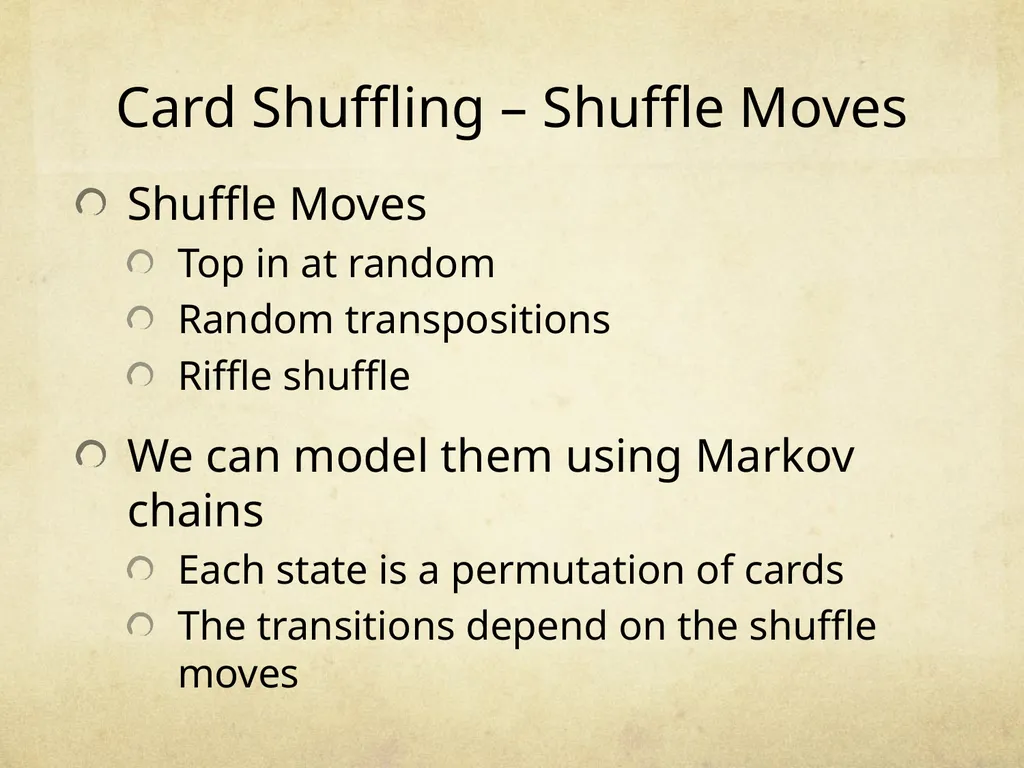
Card Shuffling – Shuffle Moves Shuffle Moves
Top in at random
Random transpositions
Riffle shuffle
We can model them using Markov chains
Each state is a permutation of cards
The transitions depend on the shuffle moves<br>
Top in at random
Random transpositions
Riffle shuffle
We can model them using Markov chains
Each state is a permutation of cards
The transitions depend on the shuffle moves<br>
81
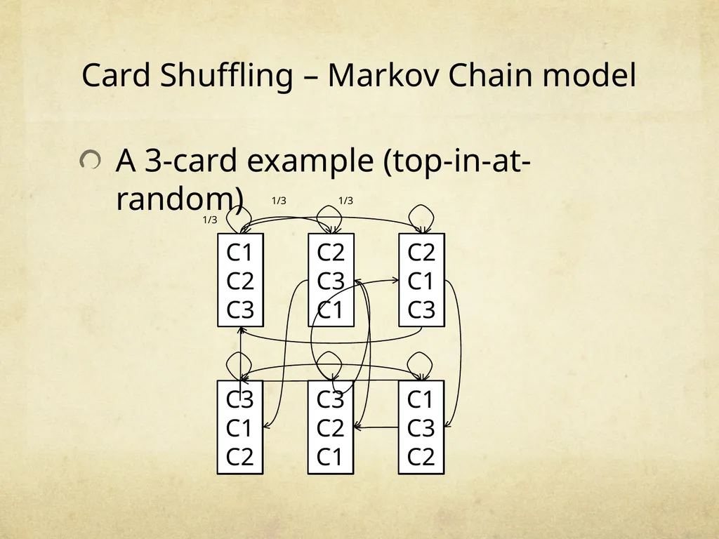
Card Shuffling – Markov Chain model A 3-card example (top-in-at-random) C1
C2
C3 C2
C3
C1 C2
C1
C3 C3
C1
C2 C3
C2
C1 C1
C3
C2<br>
C2
C3 C2
C3
C1 C2
C1
C3 C3
C1
C2 C3
C2
C1 C1
C3
C2<br>
82
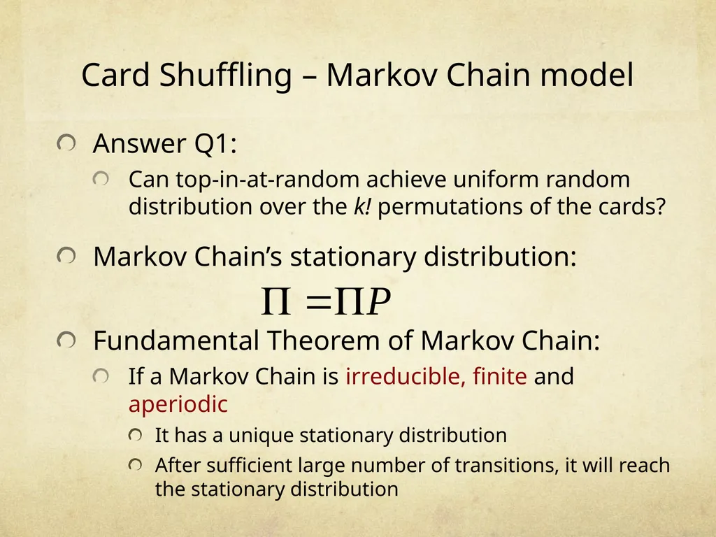
Card Shuffling – Markov Chain model Answer Q1:
Can top-in-at-random achieve uniform random distribution over the k! permutations of the cards?
Markov Chain’s stationary distribution:
Fundamental Theorem of Markov Chain:
If a Markov Chain is irreducible, finite and aperiodic
It has a unique stationary distribution
After sufficient large number of transitions, it will reach the stationary distribution<br>
Can top-in-at-random achieve uniform random distribution over the k! permutations of the cards?
Markov Chain’s stationary distribution:
Fundamental Theorem of Markov Chain:
If a Markov Chain is irreducible, finite and aperiodic
It has a unique stationary distribution
After sufficient large number of transitions, it will reach the stationary distribution<br>
83
Card Shuffling – Markov Chain model<br>
84
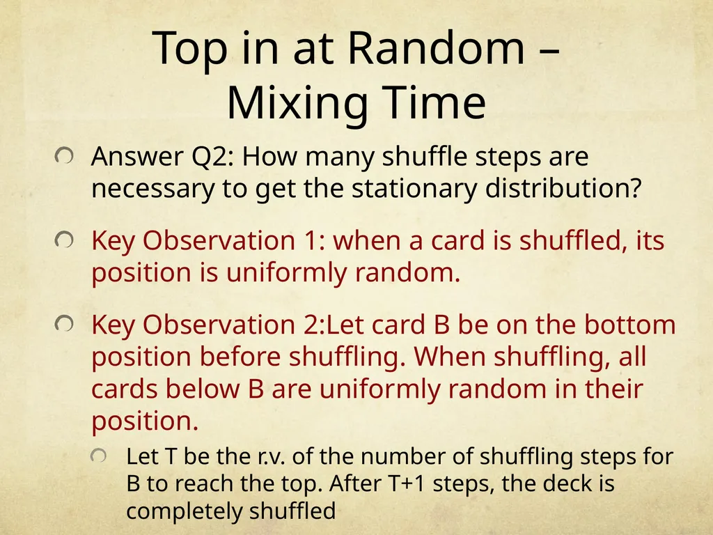
Top in at Random – Mixing Time Answer Q2: How many shuffle steps are necessary to get the stationary distribution?
Key Observation 1: when a card is shuffled, its position is uniformly random.
Key Observation 2:Let card B be on the bottom position before shuffling. When shuffling, all cards below B are uniformly random in their position.
Let T be the r.v. of the number of shuffling steps for B to reach the top. After T+1 steps, the deck is completely shuffled<br>
Key Observation 1: when a card is shuffled, its position is uniformly random.
Key Observation 2:Let card B be on the bottom position before shuffling. When shuffling, all cards below B are uniformly random in their position.
Let T be the r.v. of the number of shuffling steps for B to reach the top. After T+1 steps, the deck is completely shuffled<br>
85
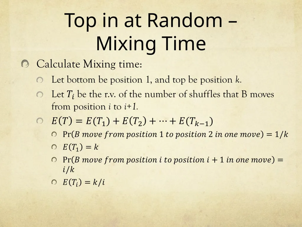
Top in at Random – Mixing Time<br>
86
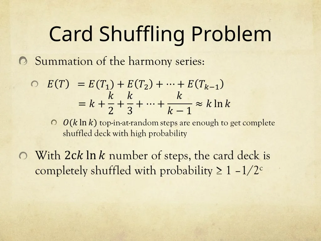
Card Shuffling Problem<br>
87
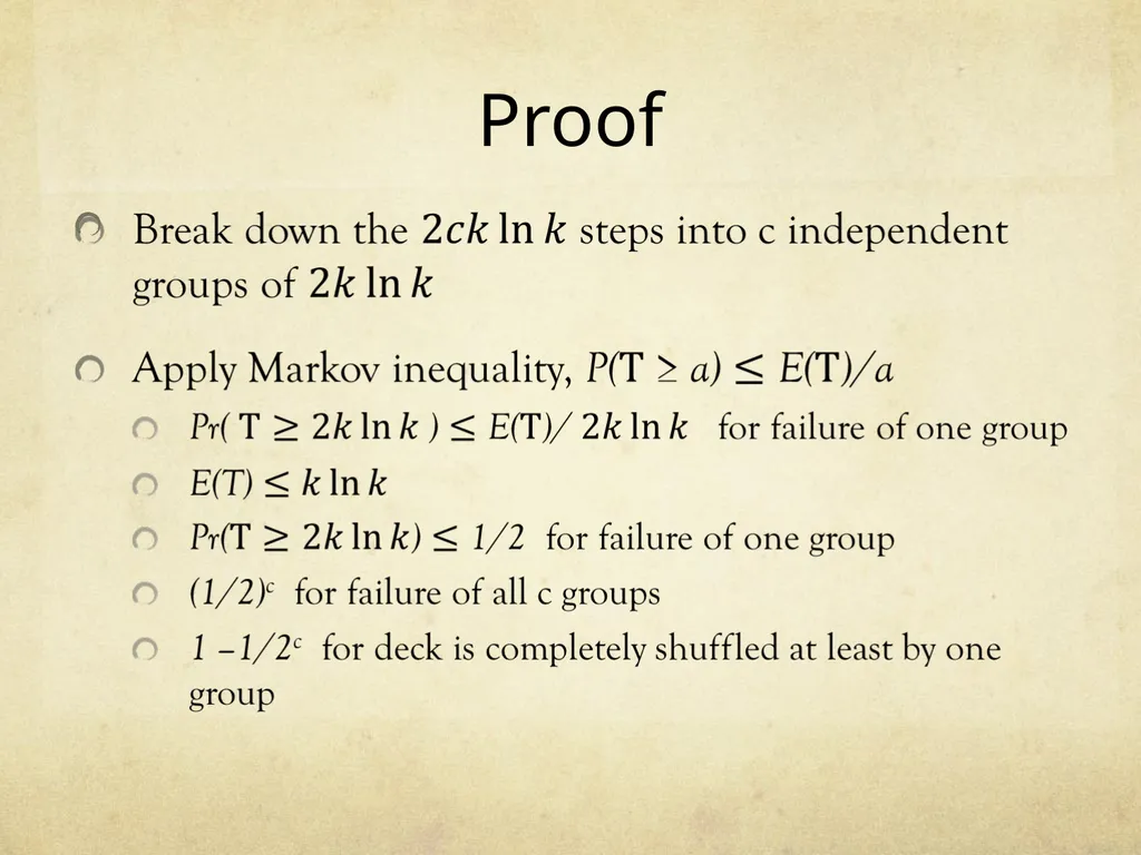
Proof<br>
88
Thank You Any Questions ?<br>
89
References Mathematics for Computer Science by Eric Lehman and Tom Leighton
Probability and Computing - Randomized Algorithms and Probabilistic Analysis by Michael Mitzenmacher and Eli Upfal
Randomized Algorithms by Rajeev Motwani and Prabhakar Raghavan
http://www.cs.berkeley.edu/~luca/cs174/notes/note8.ps
http://www.cs.berkeley.edu/~luca/cs174/notes/note9.ps<br>
Probability and Computing - Randomized Algorithms and Probabilistic Analysis by Michael Mitzenmacher and Eli Upfal
Randomized Algorithms by Rajeev Motwani and Prabhakar Raghavan
http://www.cs.berkeley.edu/~luca/cs174/notes/note8.ps
http://www.cs.berkeley.edu/~luca/cs174/notes/note9.ps<br>