S1: Chapter 8 Discrete Random Variables www.drfrostmaths.com Dr J Frost (jfrosttiffin.kingston.sch.uk) Last modified: 12th January 2016 In Chapter 2, we saw that just like in algebra, we can use a variable to represent some quantity, such
"S1: Chapter 8 Discrete Random Variables" is the property of its rightful owner. Permission is granted to
download and print the materials on this website for personal, non-commercial use only, and to display it
on your personal computer provided you do not modify the materials and that you retain all copyright
notices contained in the materials. By downloading content from our website, you accept the terms of this
agreement.
Presentation Transcript
01
S1: Chapter 8 Discrete Random Variables www.drfrostmaths.com
Dr J Frost (jfrost@tiffin.kingston.sch.uk) Last modified: 12th January 2016<br>
02
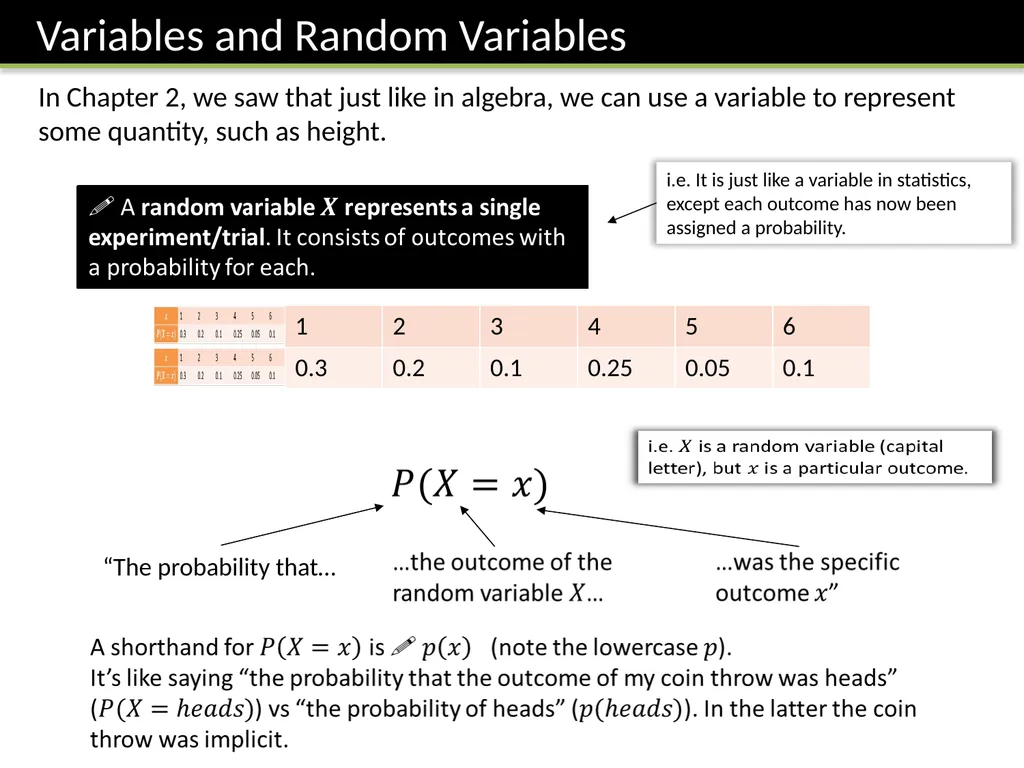
In Chapter 2, we saw that just like in algebra, we can use a variable to represent some quantity, such as height. i.e. It is just like a variable in statistics, except each outcome has now been assigned a probability. “The probability that…<br>
03
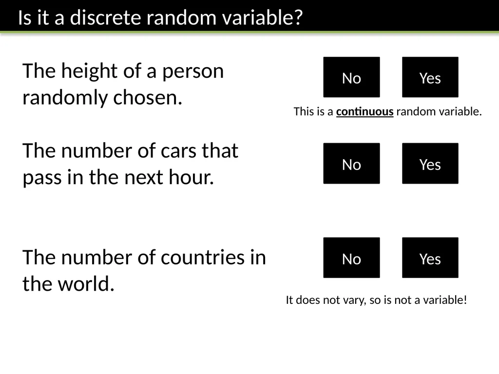
The height of a person randomly chosen.
The number of cars that pass in the next hour.
The number of countries in the world. No Yes No Yes No Yes This is a continuous random variable. It does not vary, so is not a variable!<br>
04
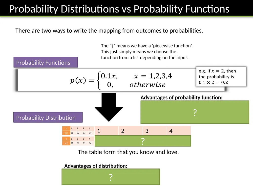
There are two ways to write the mapping from outcomes to probabilities. Probability Functions The “{“ means we have a ‘piecewise function’. This just simply means we choose the function from a list depending on the input. ? Probability Distribution The table form that you know and love. Advantages of probability function:
Can have a rule/expression based on the outcome. Particularly for continuous random variables (in S2), it would be impossible to list the probability for every outcome. More compact. Advantages of distribution:
Probability for each outcome more explicit. ? ?<br>
05
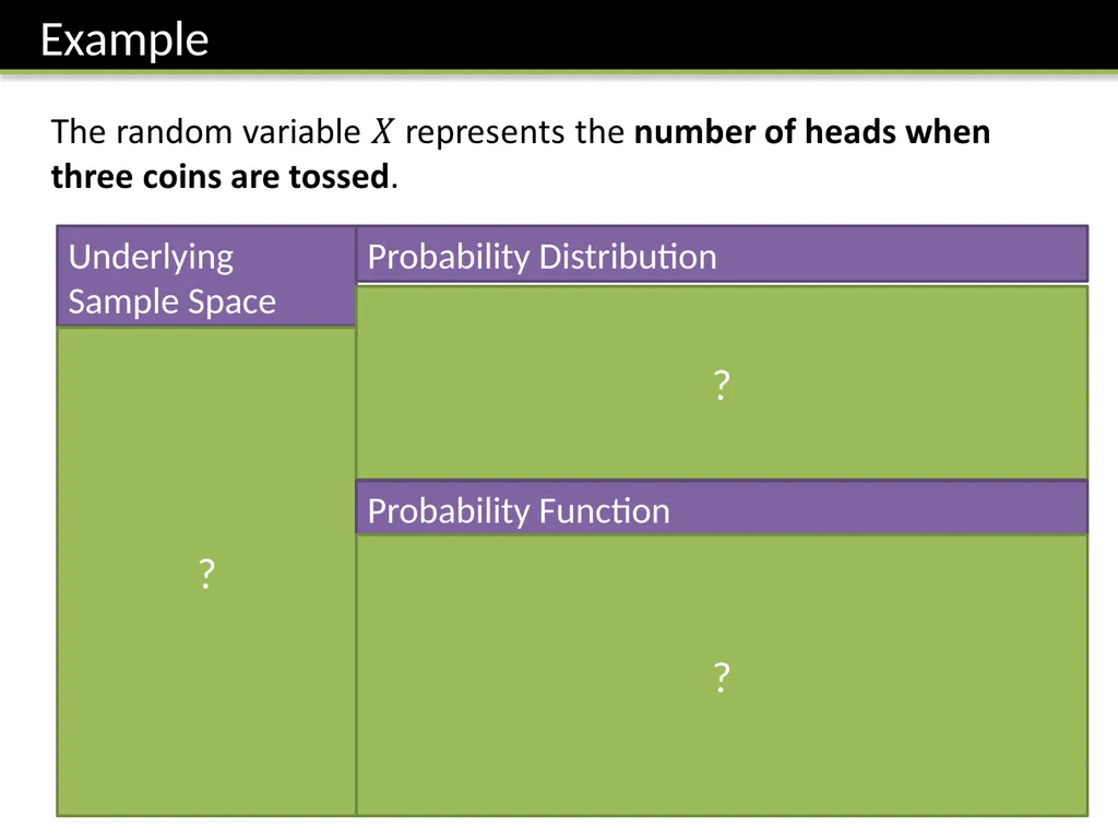
Underlying Sample Space { HHH,
HHT,
HTT,
HTH,
THH,
THT,
TTH,
TTT } Probability Distribution ? ? Probability Function ?<br>
06
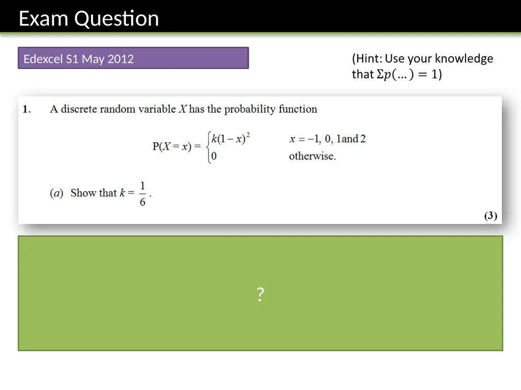
Edexcel S1 May 2012 ?<br>
07
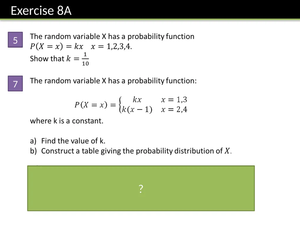
5 7 ?<br>
08
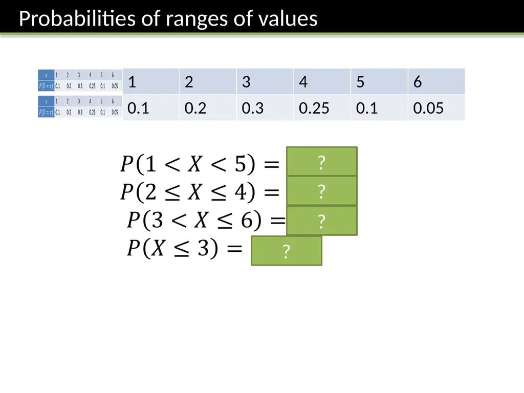
? ? ? ?<br>
09
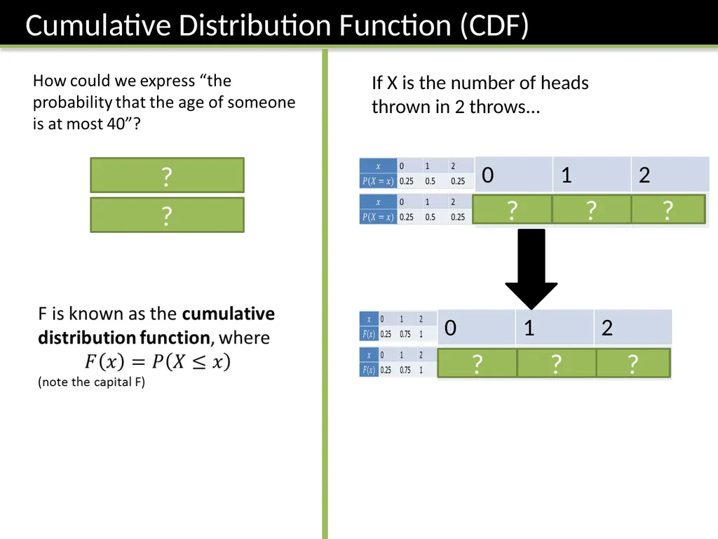
? ? If X is the number of heads thrown in 2 throws... ? ? ? ? ? ?<br>
10
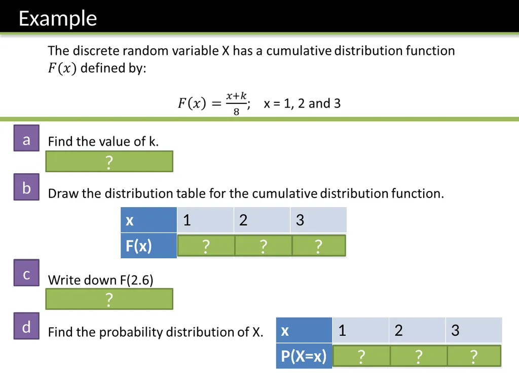
? ? ? a b c d ? ? ? ? ?<br>
11
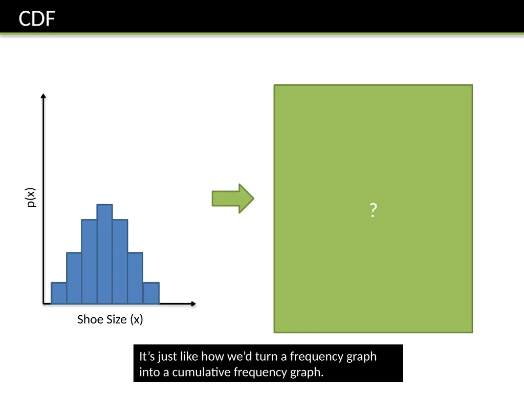
Shoe Size (x) p(x) Shoe Size (x) F(x) 1 It’s just like how we’d turn a frequency graph into a cumulative frequency graph. ?<br>
12
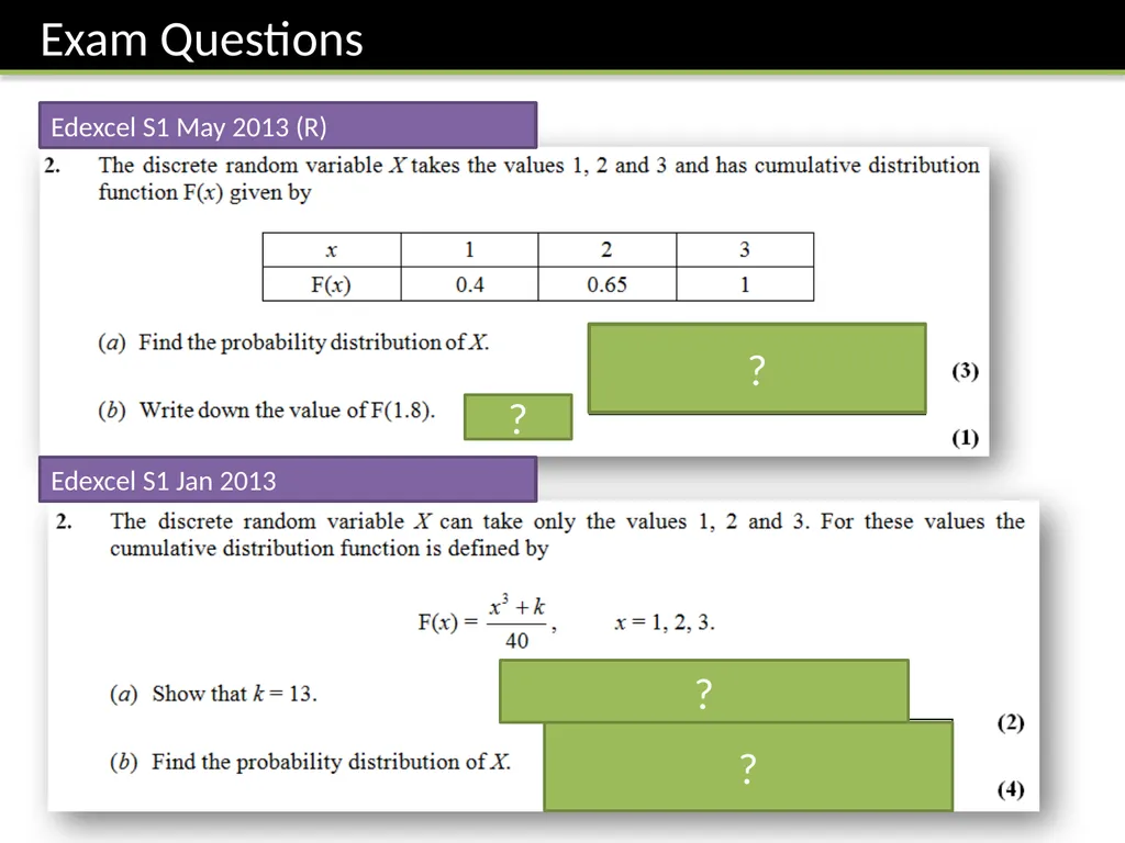
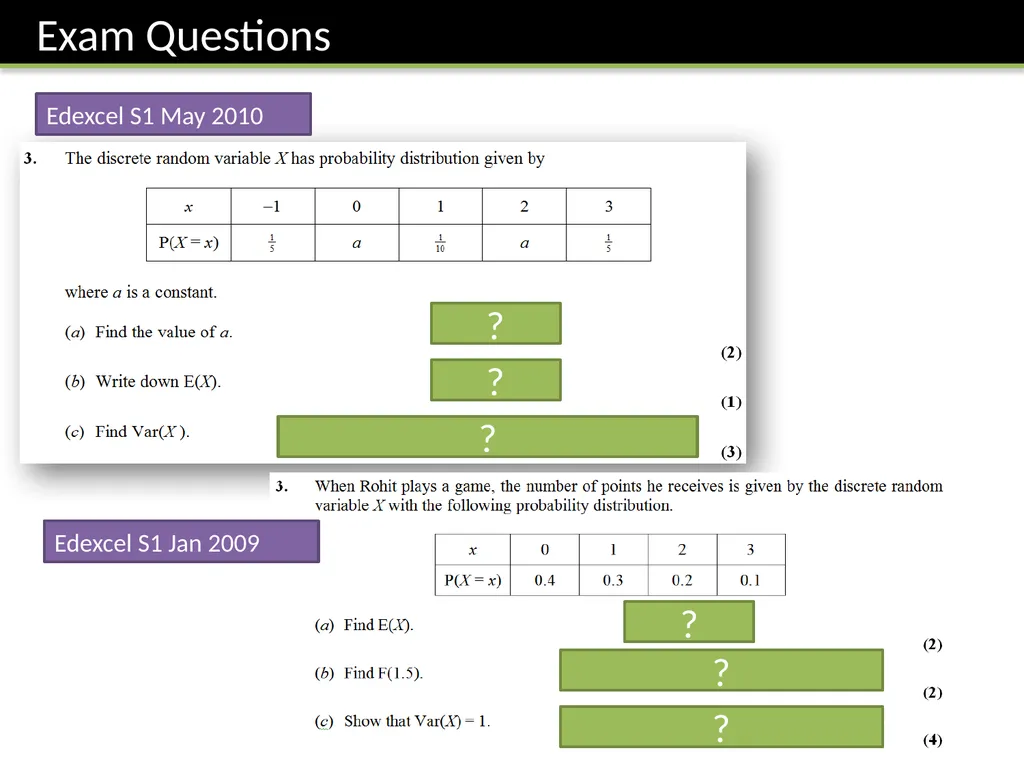
Edexcel S1 May 2013 (R) = 0.4 ? ? Edexcel S1 Jan 2013 F(3) = 1, so (27 + k)/40 = 1, ... ? ?<br>
13
Q5-8<br>
14
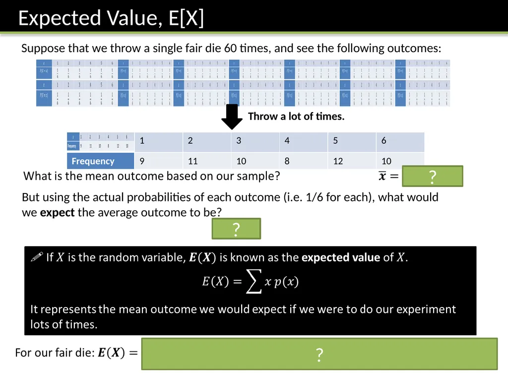
Suppose that we throw a single fair die 60 times, and see the following outcomes: But using the actual probabilities of each outcome (i.e. 1/6 for each), what would we expect the average outcome to be?
3.5 ? ? Throw a lot of times. ?<br>
15
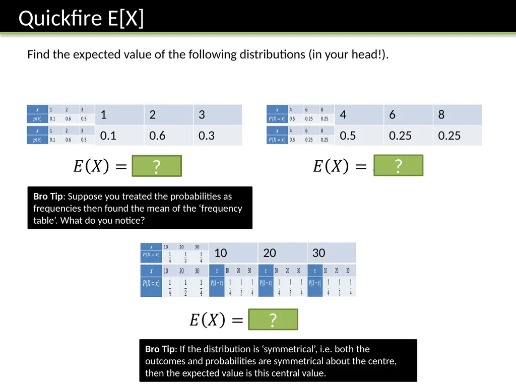
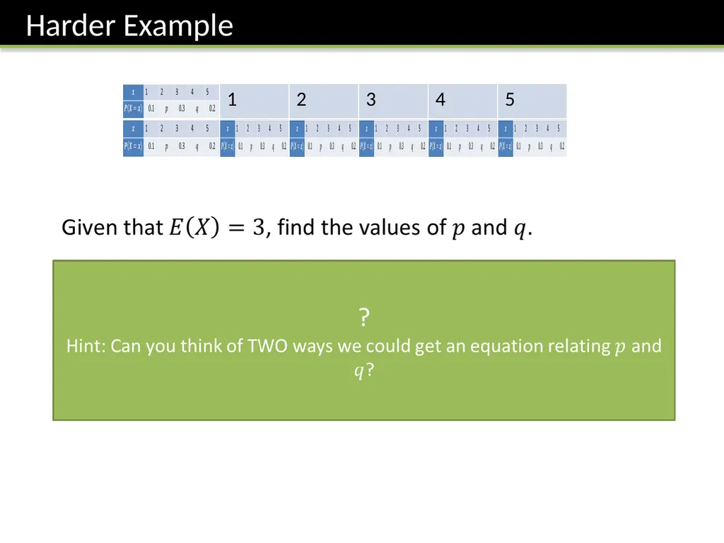
Find the expected value of the following distributions (in your head!). ? ? ? Bro Tip: Suppose you treated the probabilities as frequencies then found the mean of the ‘frequency table’. What do you notice? Bro Tip: If the distribution is ‘symmetrical’, i.e. both the outcomes and probabilities are symmetrical about the centre, then the expected value is this central value.<br>
16
? ?<br>
17
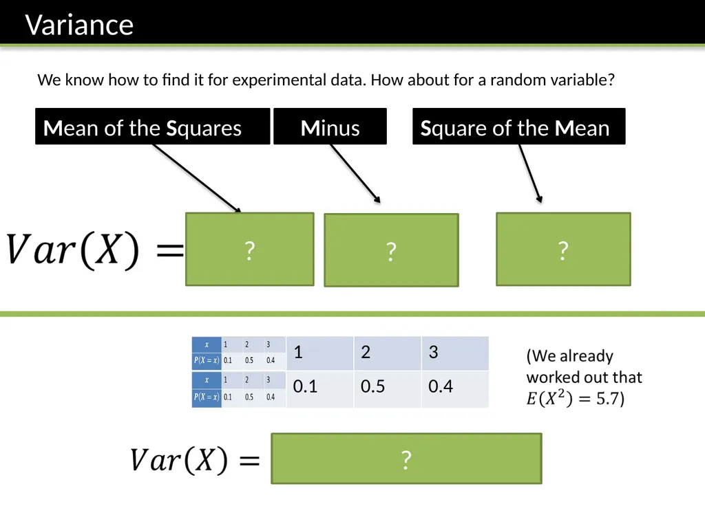
We know how to find it for experimental data. How about for a random variable? Mean of the Squares Minus Square of the Mean – ? ? ? ?<br>
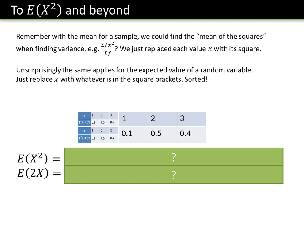
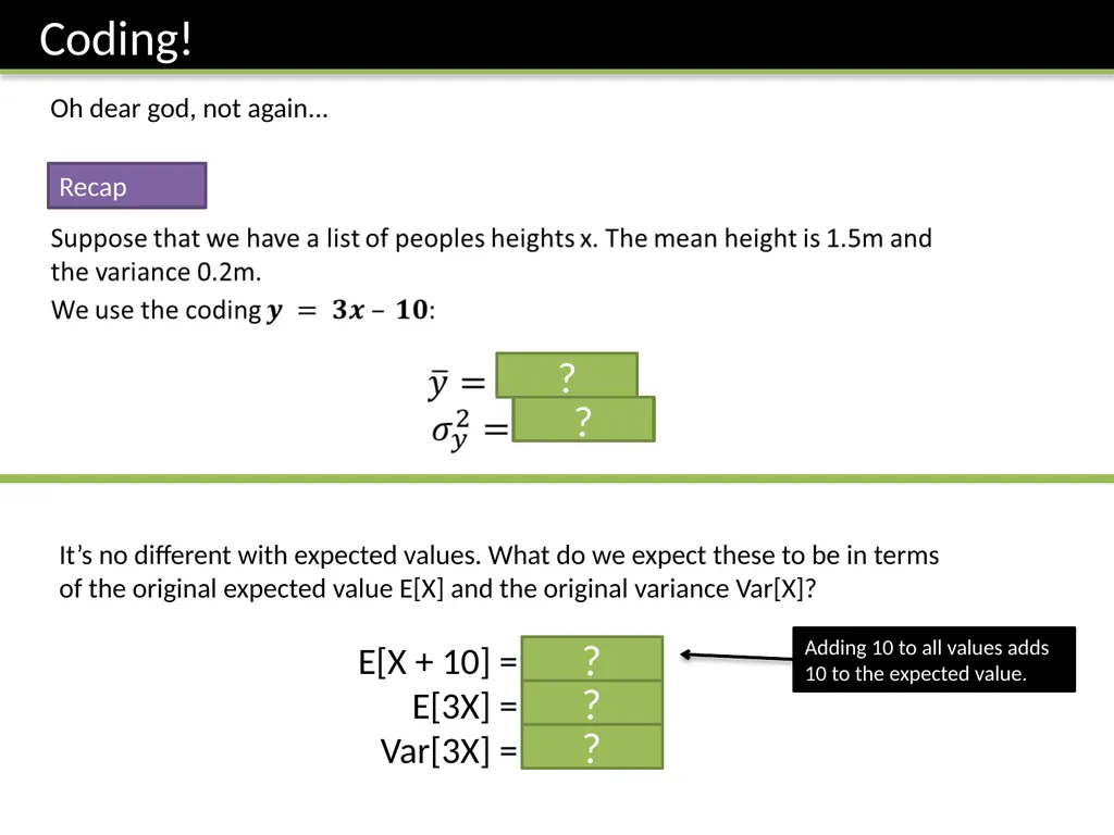
Oh dear god, not again... Recap It’s no different with expected values. What do we expect these to be in terms of the original expected value E[X] and the original variance Var[X]?
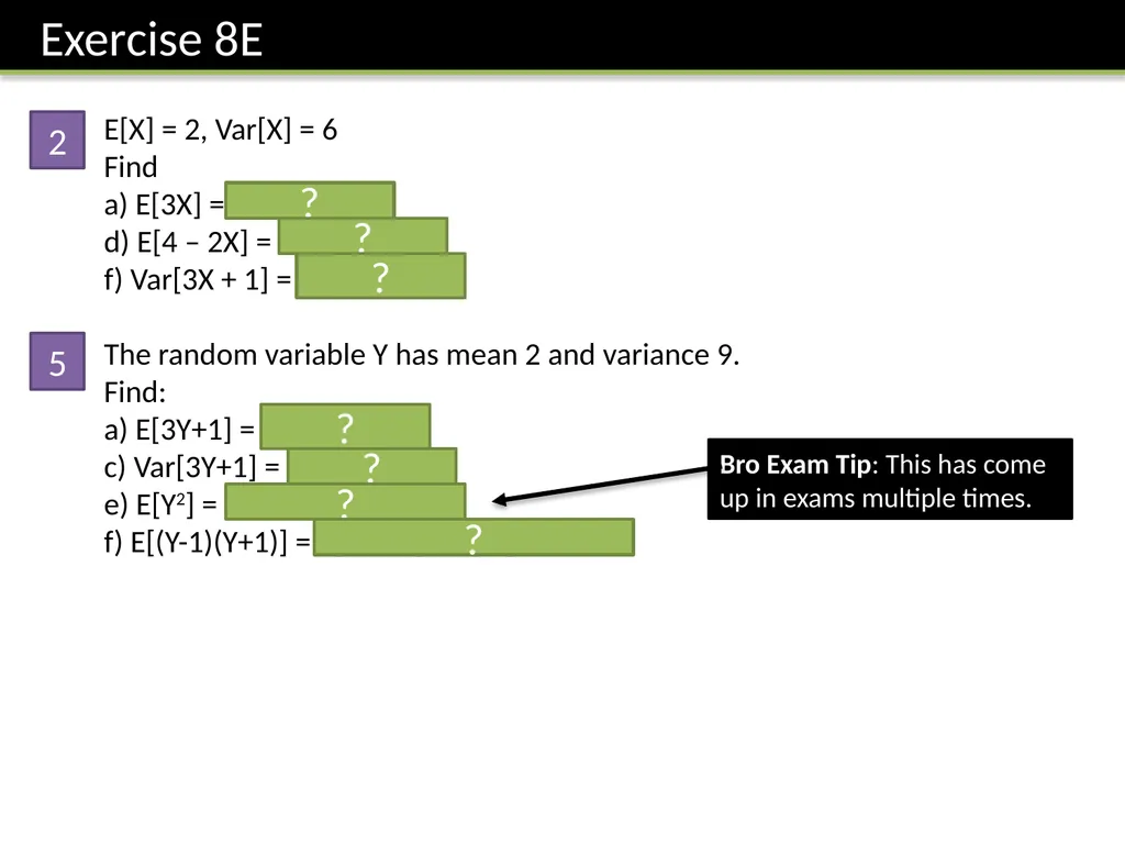
The random variable Y has mean 2 and variance 9.
Find:
a) E[3Y+1] = 3E[Y] + 1 = 7
c) Var[3Y+1] = 9Var[Y] = 81
e) E[Y2] = Var[Y] + E[Y]2 = 13
f) E[(Y-1)(Y+1)] = E[Y2 – 1] = E[Y2] – 1 = 12 2 5 ? ? ? ? ? ? ? Bro Exam Tip: This has come up in exams multiple times.<br>
22
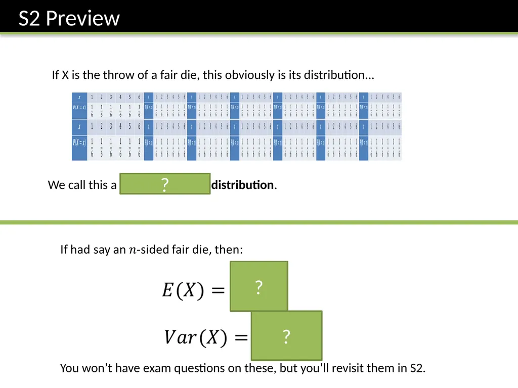
If X is the throw of a fair die, this obviously is its distribution... We call this a discrete uniform distribution. ? You won’t have exam questions on these, but you’ll revisit them in S2. ? ?<br>