
Search Advertising These slides are modified from
TA
Published · 28 slides · 0 views

1 / 1
Description
Search Advertising These slides are modified from those by Anand Rajaram Jeff Ullman History of web advertising Banner ads (1995-2001) Initial form of web advertising Popular websites charged X for every 1000 impressions of ad Called
Related Topics
Share
Embed code
Download this presentation From Below
"Search Advertising These slides are modified from" is the property of its rightful owner. Permission is granted to download and print the materials on this website for personal, non-commercial use only, and to display it on your personal computer provided you do not modify the materials and that you retain all copyright notices contained in the materials. By downloading content from our website, you accept the terms of this agreement.
Presentation Transcript
01
Search Advertising These slides are modified from those by Anand Rajaram & Jeff Ullman<br>
02
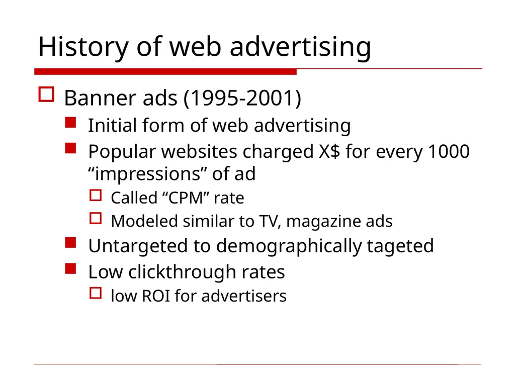
History of web advertising Banner ads (1995-2001)
Initial form of web advertising
Popular websites charged X$ for every 1000 “impressions” of ad
Called “CPM” rate
Modeled similar to TV, magazine ads
Untargeted to demographically tageted
Low clickthrough rates
low ROI for advertisers<br>
Initial form of web advertising
Popular websites charged X$ for every 1000 “impressions” of ad
Called “CPM” rate
Modeled similar to TV, magazine ads
Untargeted to demographically tageted
Low clickthrough rates
low ROI for advertisers<br>
03
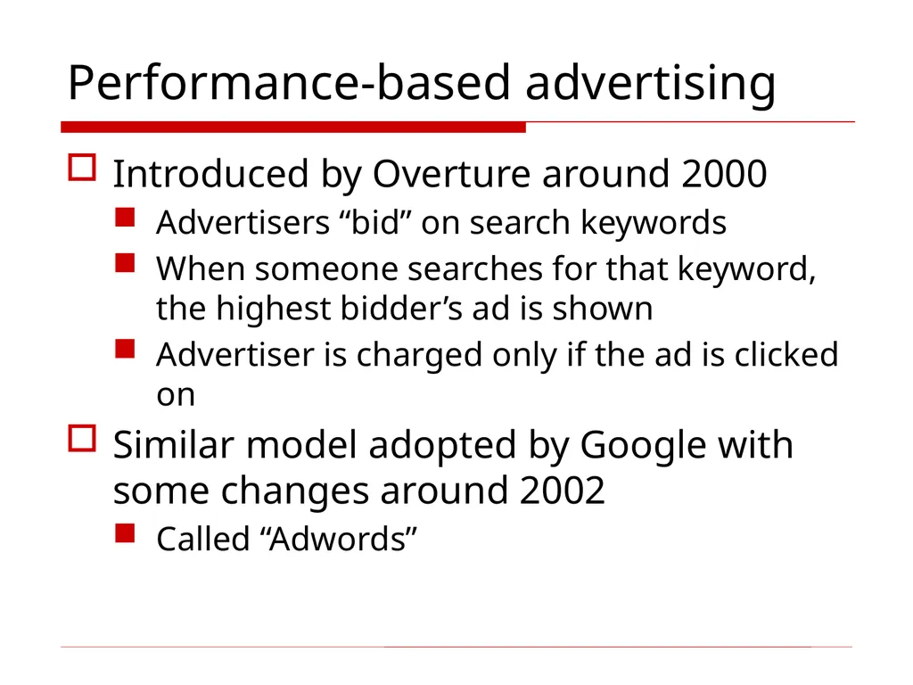
Performance-based advertising Introduced by Overture around 2000
Advertisers “bid” on search keywords
When someone searches for that keyword, the highest bidder’s ad is shown
Advertiser is charged only if the ad is clicked on
Similar model adopted by Google with some changes around 2002
Called “Adwords”<br>
Advertisers “bid” on search keywords
When someone searches for that keyword, the highest bidder’s ad is shown
Advertiser is charged only if the ad is clicked on
Similar model adopted by Google with some changes around 2002
Called “Adwords”<br>
04
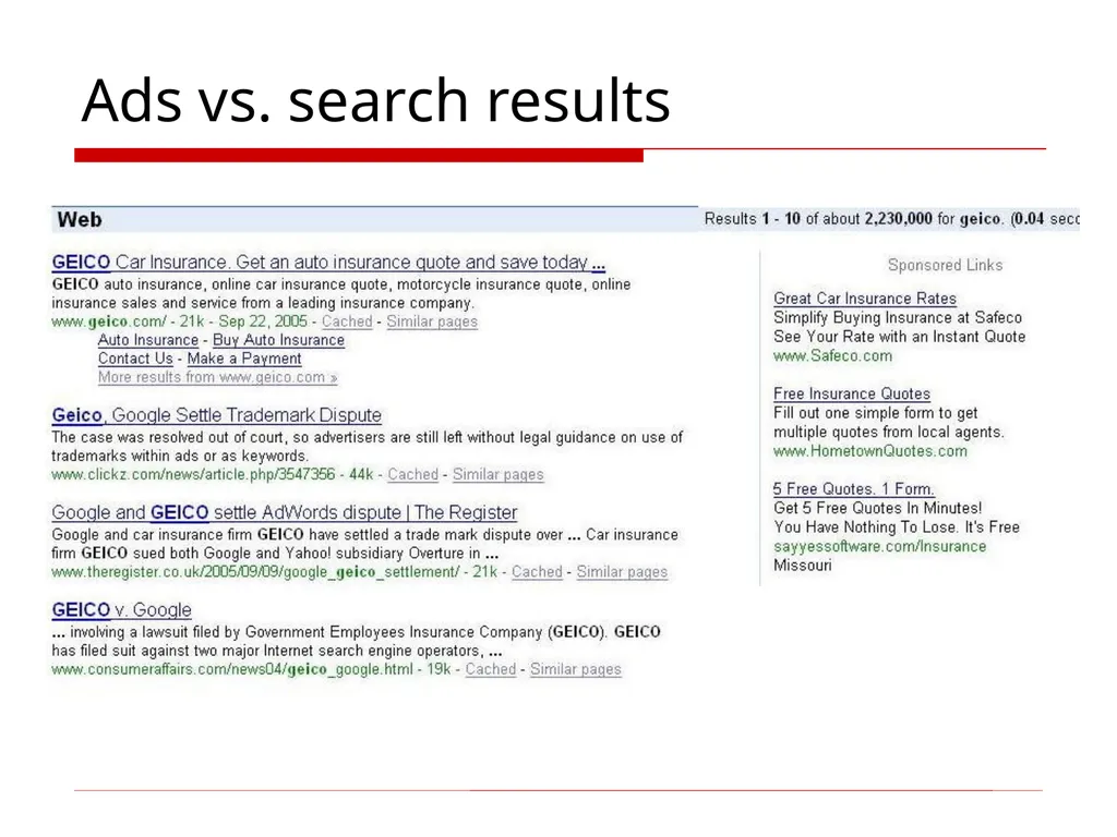
Ads vs. search results<br>
05
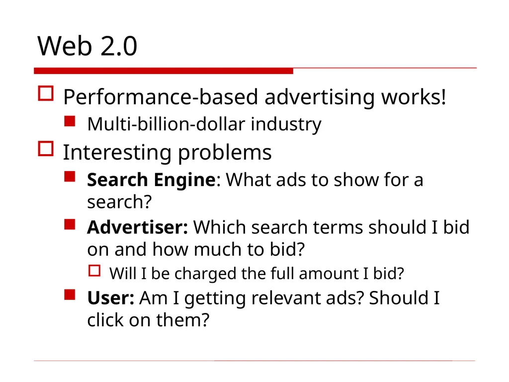
Web 2.0 Performance-based advertising works!
Multi-billion-dollar industry
Interesting problems
Search Engine: What ads to show for a search?
Advertiser: Which search terms should I bid on and how much to bid?
Will I be charged the full amount I bid?
User: Am I getting relevant ads? Should I click on them?<br>
Multi-billion-dollar industry
Interesting problems
Search Engine: What ads to show for a search?
Advertiser: Which search terms should I bid on and how much to bid?
Will I be charged the full amount I bid?
User: Am I getting relevant ads? Should I click on them?<br>
06
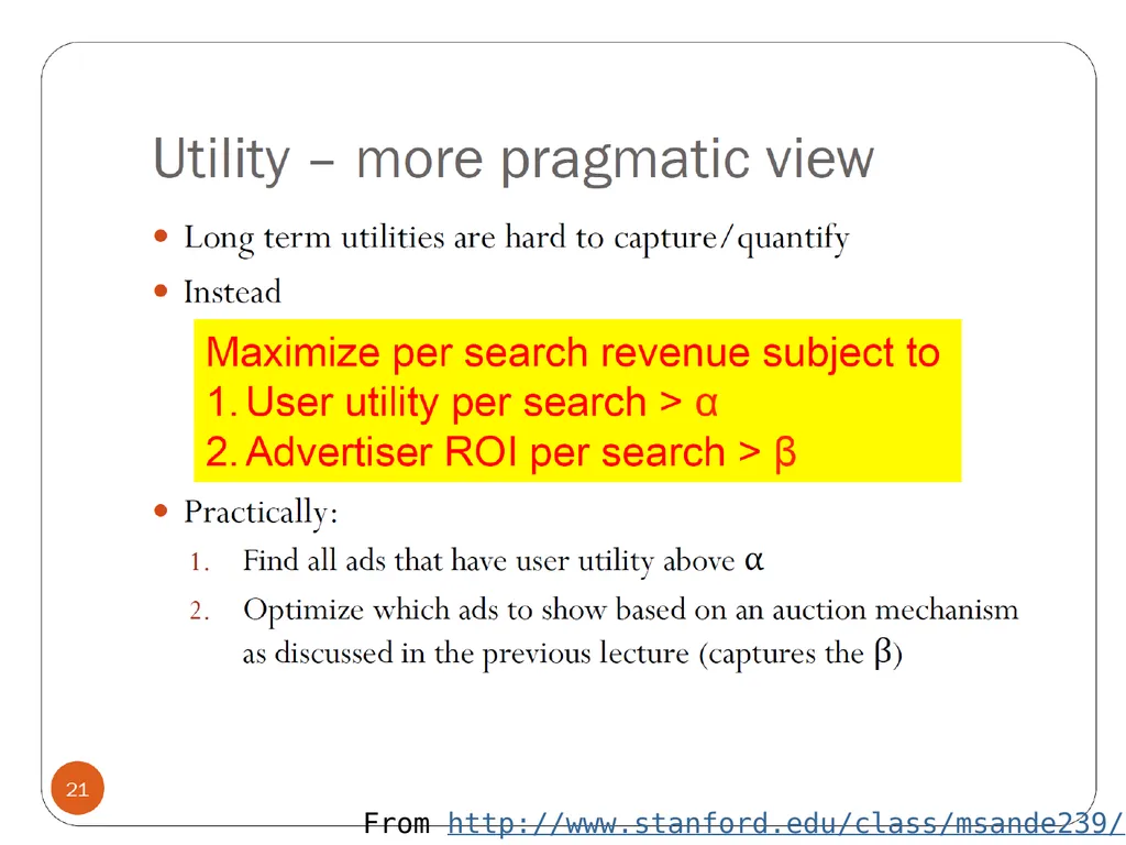
From http://www.stanford.edu/class/msande239/<br>
07
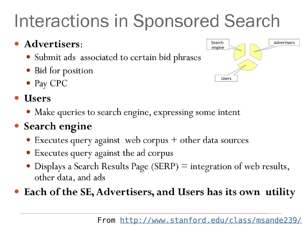
From http://www.stanford.edu/class/msande239/<br>
08
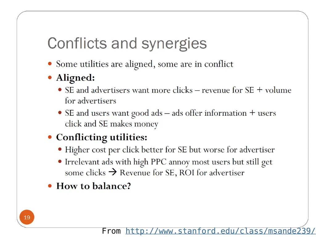
From http://www.stanford.edu/class/msande239/<br>
09
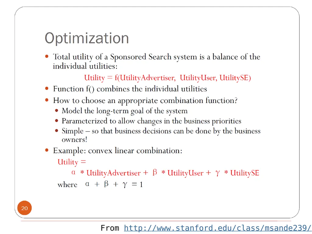
From http://www.stanford.edu/class/msande239/<br>
10
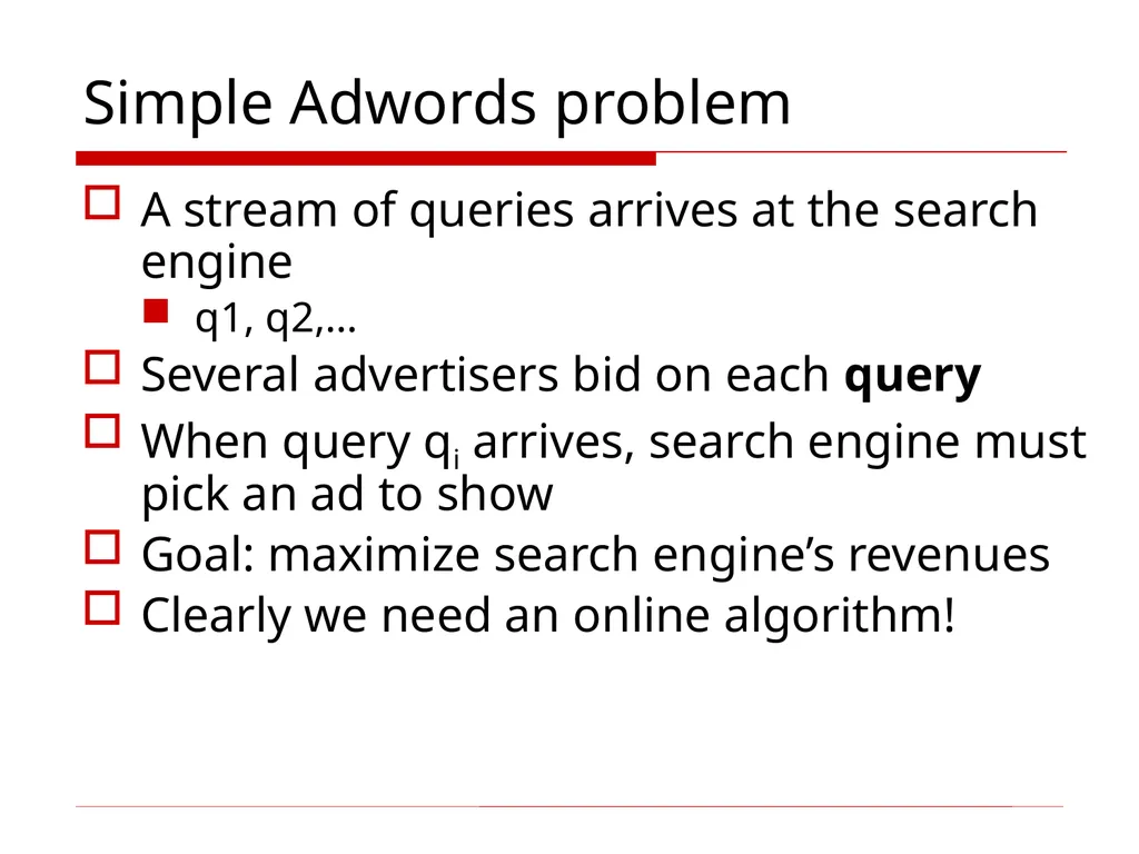
Simple Adwords problem A stream of queries arrives at the search engine
q1, q2,…
Several advertisers bid on each query
When query qi arrives, search engine must pick an ad to show
Goal: maximize search engine’s revenues
Clearly we need an online algorithm!<br>
q1, q2,…
Several advertisers bid on each query
When query qi arrives, search engine must pick an ad to show
Goal: maximize search engine’s revenues
Clearly we need an online algorithm!<br>
11
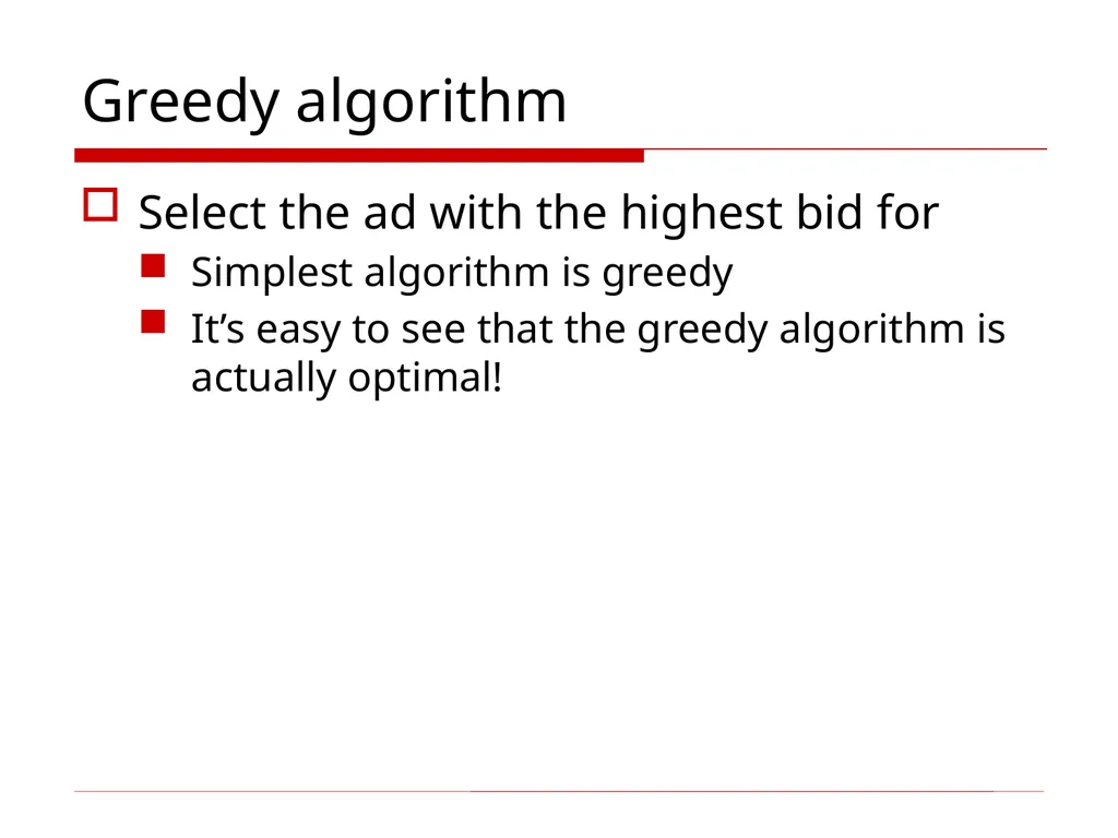
Greedy algorithm Select the ad with the highest bid for
Simplest algorithm is greedy
It’s easy to see that the greedy algorithm is actually optimal!<br>
Simplest algorithm is greedy
It’s easy to see that the greedy algorithm is actually optimal!<br>
12
Complication 1:
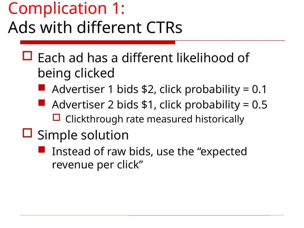
Ads with different CTRs Each ad has a different likelihood of being clicked
Advertiser 1 bids $2, click probability = 0.1
Advertiser 2 bids $1, click probability = 0.5
Clickthrough rate measured historically
Simple solution
Instead of raw bids, use the “expected revenue per click”<br>
Advertiser 1 bids $2, click probability = 0.1
Advertiser 2 bids $1, click probability = 0.5
Clickthrough rate measured historically
Simple solution
Instead of raw bids, use the “expected revenue per click”<br>
13
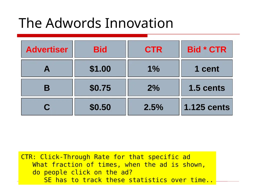
The Adwords Innovation Advertiser Bid CTR Bid * CTR A B C $1.00 $0.75 $0.50 1% 2% 2.5% 1 cent 1.5 cents 1.125 cents CTR: Click-Through Rate for that specific ad
What fraction of times, when the ad is shown,
do people click on the ad?
SE has to track these statistics over time..<br>
What fraction of times, when the ad is shown,
do people click on the ad?
SE has to track these statistics over time..<br>
14
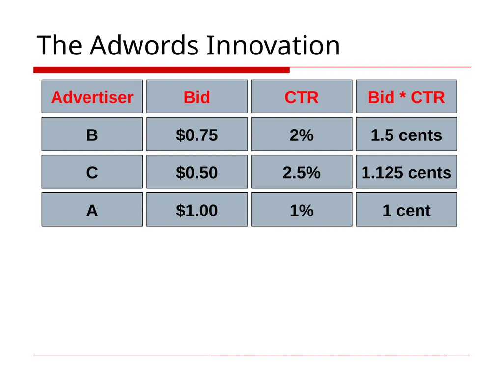
The Adwords Innovation Advertiser Bid CTR Bid * CTR A B C $1.00 $0.75 $0.50 1% 2% 2.5% 1 cent 1.5 cents 1.125 cents<br>
15
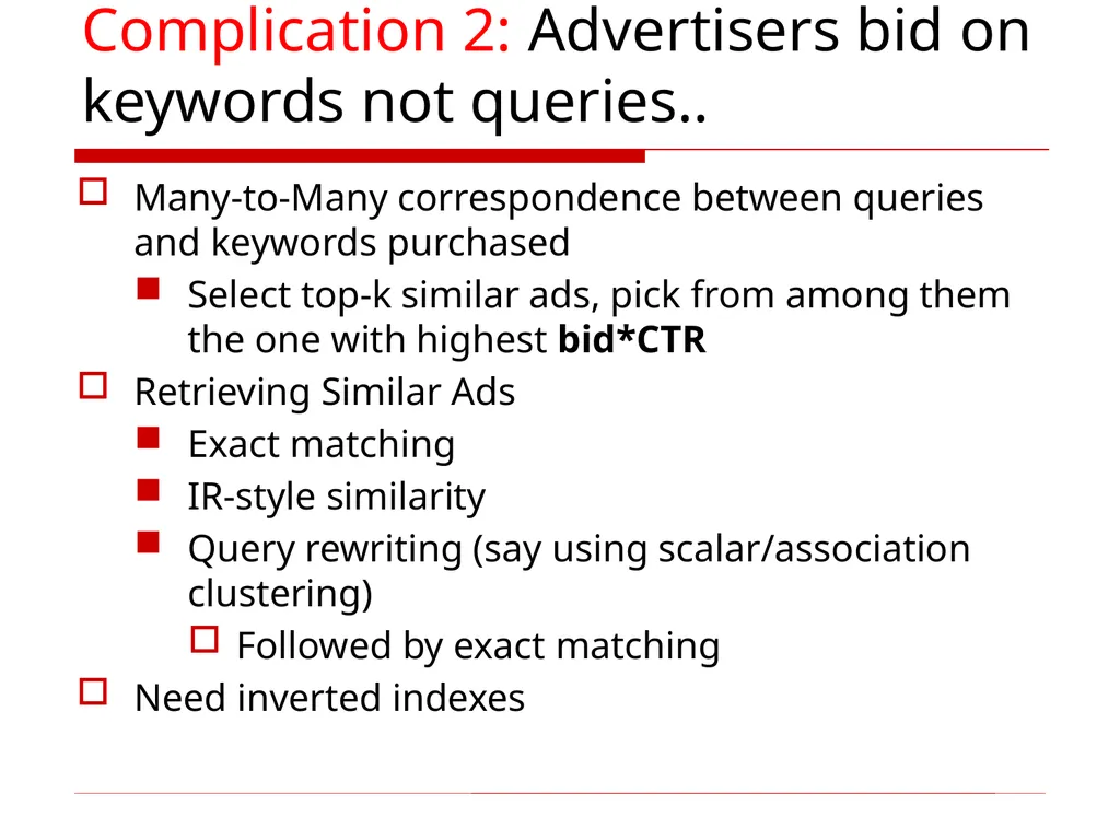
Complication 2: Advertisers bid on keywords not queries.. Many-to-Many correspondence between queries and keywords purchased
Select top-k similar ads, pick from among them the one with highest bid*CTR
Retrieving Similar Ads
Exact matching
IR-style similarity
Query rewriting (say using scalar/association clustering)
Followed by exact matching
Need inverted indexes<br>
Select top-k similar ads, pick from among them the one with highest bid*CTR
Retrieving Similar Ads
Exact matching
IR-style similarity
Query rewriting (say using scalar/association clustering)
Followed by exact matching
Need inverted indexes<br>
16
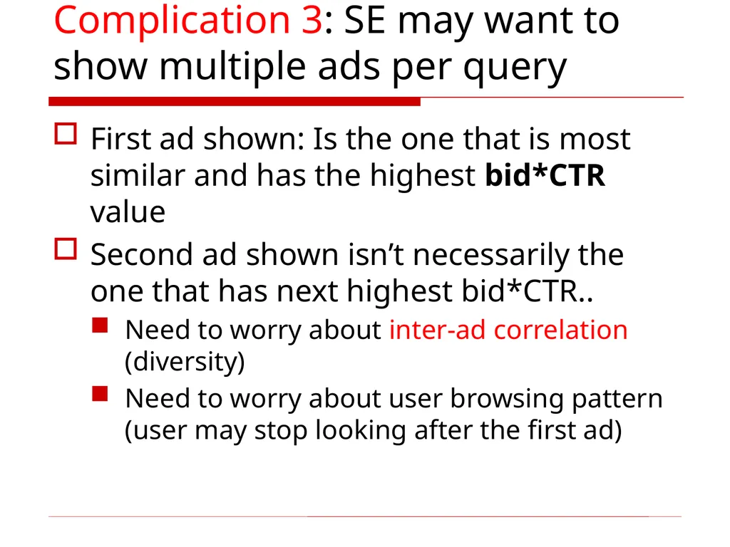
Complication 3: SE may want to show multiple ads per query First ad shown: Is the one that is most similar and has the highest bid*CTR value
Second ad shown isn’t necessarily the one that has next highest bid*CTR..
Need to worry about inter-ad correlation (diversity)
Need to worry about user browsing pattern (user may stop looking after the first ad)<br>
Second ad shown isn’t necessarily the one that has next highest bid*CTR..
Need to worry about inter-ad correlation (diversity)
Need to worry about user browsing pattern (user may stop looking after the first ad)<br>
17
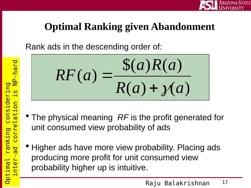
Optimal Ranking given Abandonment The physical meaning RF is the profit generated for unit consumed view probability of ads
Higher ads have more view probability. Placing ads producing more profit for unit consumed view probability higher up is intuitive. Rank ads in the descending order of: 17 Optimal ranking considering
inter-ad correlation is NP-hard Raju Balakrishnan<br>
Higher ads have more view probability. Placing ads producing more profit for unit consumed view probability higher up is intuitive. Rank ads in the descending order of: 17 Optimal ranking considering
inter-ad correlation is NP-hard Raju Balakrishnan<br>
18
Complication 4: Advertisers have limited budgets Each advertiser has a limited budget
Search engine guarantees that the advertiser will not be charged more than their daily budget
SE needs to be smarter in selecting among the relevant advertisers so it is sensitive to the remaining budget..<br>
Search engine guarantees that the advertiser will not be charged more than their daily budget
SE needs to be smarter in selecting among the relevant advertisers so it is sensitive to the remaining budget..<br>
19
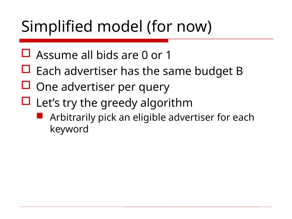
Simplified model (for now) Assume all bids are 0 or 1
Each advertiser has the same budget B
One advertiser per query
Let’s try the greedy algorithm
Arbitrarily pick an eligible advertiser for each keyword<br>
Each advertiser has the same budget B
One advertiser per query
Let’s try the greedy algorithm
Arbitrarily pick an eligible advertiser for each keyword<br>
20
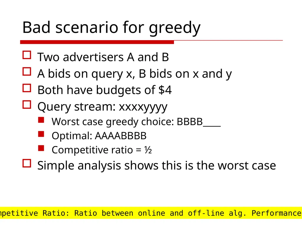
Bad scenario for greedy Two advertisers A and B
A bids on query x, B bids on x and y
Both have budgets of $4
Query stream: xxxxyyyy
Worst case greedy choice: BBBB____
Optimal: AAAABBBB
Competitive ratio = ½
Simple analysis shows this is the worst case Competitive Ratio: Ratio between online and off-line alg. Performance<br>
A bids on query x, B bids on x and y
Both have budgets of $4
Query stream: xxxxyyyy
Worst case greedy choice: BBBB____
Optimal: AAAABBBB
Competitive ratio = ½
Simple analysis shows this is the worst case Competitive Ratio: Ratio between online and off-line alg. Performance<br>
21
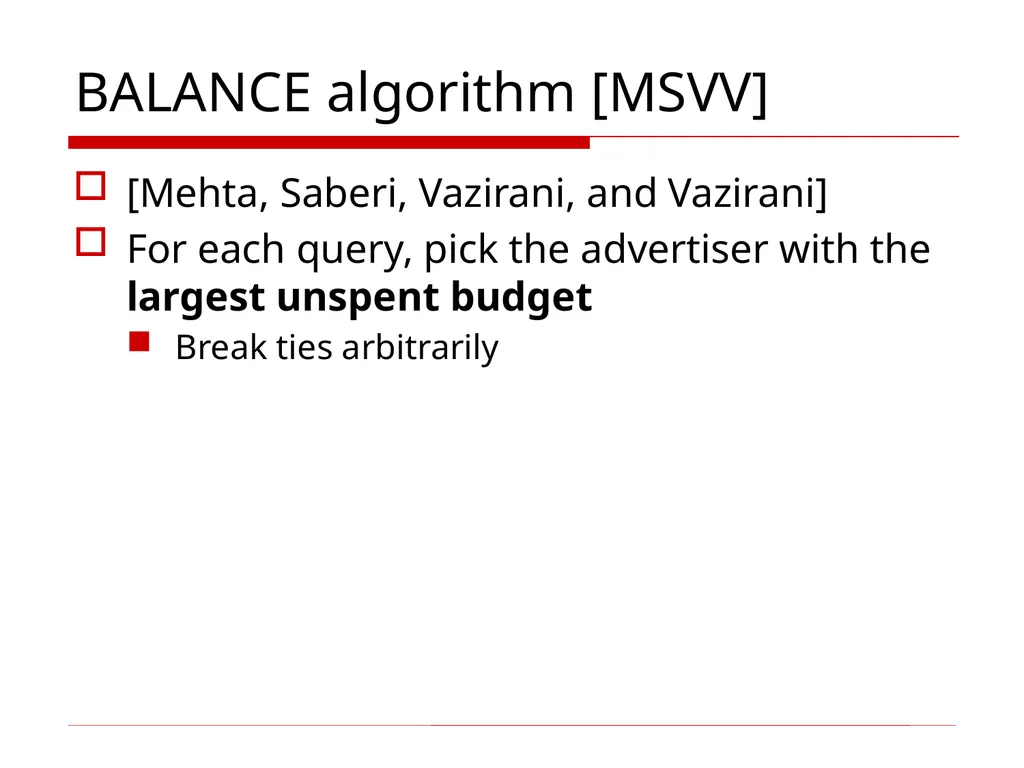
BALANCE algorithm [MSVV] [Mehta, Saberi, Vazirani, and Vazirani]
For each query, pick the advertiser with the largest unspent budget
Break ties arbitrarily<br>
For each query, pick the advertiser with the largest unspent budget
Break ties arbitrarily<br>
22
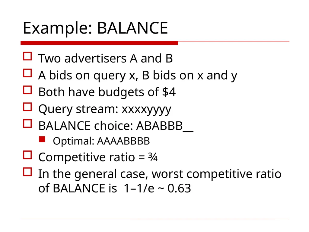
Example: BALANCE Two advertisers A and B
A bids on query x, B bids on x and y
Both have budgets of $4
Query stream: xxxxyyyy
BALANCE choice: ABABBB__
Optimal: AAAABBBB
Competitive ratio = ¾
In the general case, worst competitive ratio of BALANCE is 1–1/e ~ 0.63<br>
A bids on query x, B bids on x and y
Both have budgets of $4
Query stream: xxxxyyyy
BALANCE choice: ABABBB__
Optimal: AAAABBBB
Competitive ratio = ¾
In the general case, worst competitive ratio of BALANCE is 1–1/e ~ 0.63<br>
23
Analyzing BALANCE Consider simple case: two advertisers, A1 and A2, each with budget B (assume B À 1)
Assume optimal solution exhausts both advertisers’ budgets
BALANCE must exhaust at least one advertiser’s budget
If not, we can allocate more queries
Assume BALANCE exhausts A2’s budget<br>
Assume optimal solution exhausts both advertisers’ budgets
BALANCE must exhaust at least one advertiser’s budget
If not, we can allocate more queries
Assume BALANCE exhausts A2’s budget<br>
24
Analyzing Balance Opt revenue = 2B
Balance revenue = 2B-x = B+y We have y ¸ x
Balance revenue is minimum for x=y=B/2
Minimum Balance revenue = 3B/2
Competitive Ratio = 3/4 Queries allocated to A1 in optimal solution Queries allocated to A2 in optimal solution<br>
Balance revenue = 2B-x = B+y We have y ¸ x
Balance revenue is minimum for x=y=B/2
Minimum Balance revenue = 3B/2
Competitive Ratio = 3/4 Queries allocated to A1 in optimal solution Queries allocated to A2 in optimal solution<br>
25
General Result In the general case, worst competitive ratio of BALANCE is 1–1/e = approx. 0.63
Interestingly, no online algorithm has a better competitive ratio
Won’t go through the details here, but let’s see the worst case that gives this ratio<br>
Interestingly, no online algorithm has a better competitive ratio
Won’t go through the details here, but let’s see the worst case that gives this ratio<br>
26
Worst case for BALANCE N advertisers, each with budget B À N À 1
NB queries appear in N rounds of B queries each
Round 1 queries: bidders A1, A2, …, AN
Round 2 queries: bidders A2, A3, …, AN
Round i queries: bidders Ai, …, AN
Optimum allocation: allocate round i queries to Ai
Optimum revenue NB<br>
NB queries appear in N rounds of B queries each
Round 1 queries: bidders A1, A2, …, AN
Round 2 queries: bidders A2, A3, …, AN
Round i queries: bidders Ai, …, AN
Optimum allocation: allocate round i queries to Ai
Optimum revenue NB<br>
27
BALANCE allocation … A1 A2 A3 AN-1 AN After k rounds, sum of allocations to each of bins Ak,…,AN is
Sk = Sk+1 = … = SN = 1· 1· kB/(N-i+1) If we find the smallest k such that Sk ¸ B, then after k rounds
we cannot allocate any queries to any advertiser<br>
Sk = Sk+1 = … = SN = 1· 1· kB/(N-i+1) If we find the smallest k such that Sk ¸ B, then after k rounds
we cannot allocate any queries to any advertiser<br>
28
BALANCE analysis B/1 B/2 B/3 … B/(N-k+1) … B/(N-1) B/N S1 S2 Sk = B<br>
29
BALANCE analysis Fact: Hn = 1· i· n1/i = approx. log(n) for large n
Result due to Euler 1/1 1/2 1/3 … 1/(N-k+1) … 1/(N-1) 1/N log(N) Sk = 1 implies HN-k = log(N)-1 = log(N/e)
N-k = N/e
k = N(1-1/e)<br>
Result due to Euler 1/1 1/2 1/3 … 1/(N-k+1) … 1/(N-1) 1/N log(N) Sk = 1 implies HN-k = log(N)-1 = log(N/e)
N-k = N/e
k = N(1-1/e)<br>
30
BALANCE analysis So after the first N(1-1/e) rounds, we cannot allocate a query to any advertiser
Revenue = BN(1-1/e)
Competitive ratio = 1-1/e<br>
Revenue = BN(1-1/e)
Competitive ratio = 1-1/e<br>
31
General version of problem Arbitrary bids, budgets
Consider query q, advertiser i
Bid = xi
Budget = bi
BALANCE can be terrible
Consider two advertisers A1 and A2
A1: x1 = 1, b1 = 110
A2: x2 = 10, b2 = 100<br>
Consider query q, advertiser i
Bid = xi
Budget = bi
BALANCE can be terrible
Consider two advertisers A1 and A2
A1: x1 = 1, b1 = 110
A2: x2 = 10, b2 = 100<br>
32
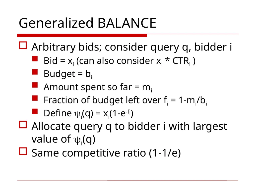
Generalized BALANCE Arbitrary bids; consider query q, bidder i
Bid = xi (can also consider xi * CTRi )
Budget = bi
Amount spent so far = mi
Fraction of budget left over fi = 1-mi/bi
Define i(q) = xi(1-e-fi)
Allocate query q to bidder i with largest value of i(q)
Same competitive ratio (1-1/e)<br>
Bid = xi (can also consider xi * CTRi )
Budget = bi
Amount spent so far = mi
Fraction of budget left over fi = 1-mi/bi
Define i(q) = xi(1-e-fi)
Allocate query q to bidder i with largest value of i(q)
Same competitive ratio (1-1/e)<br>
33
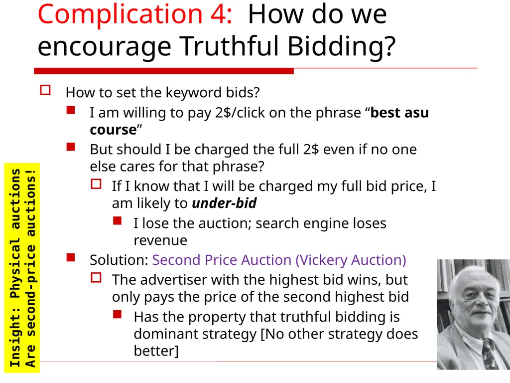
Complication 4: How do we encourage Truthful Bidding? How to set the keyword bids?
I am willing to pay 2$/click on the phrase “best asu course”
But should I be charged the full 2$ even if no one else cares for that phrase?
If I know that I will be charged my full bid price, I am likely to under-bid
I lose the auction; search engine loses revenue
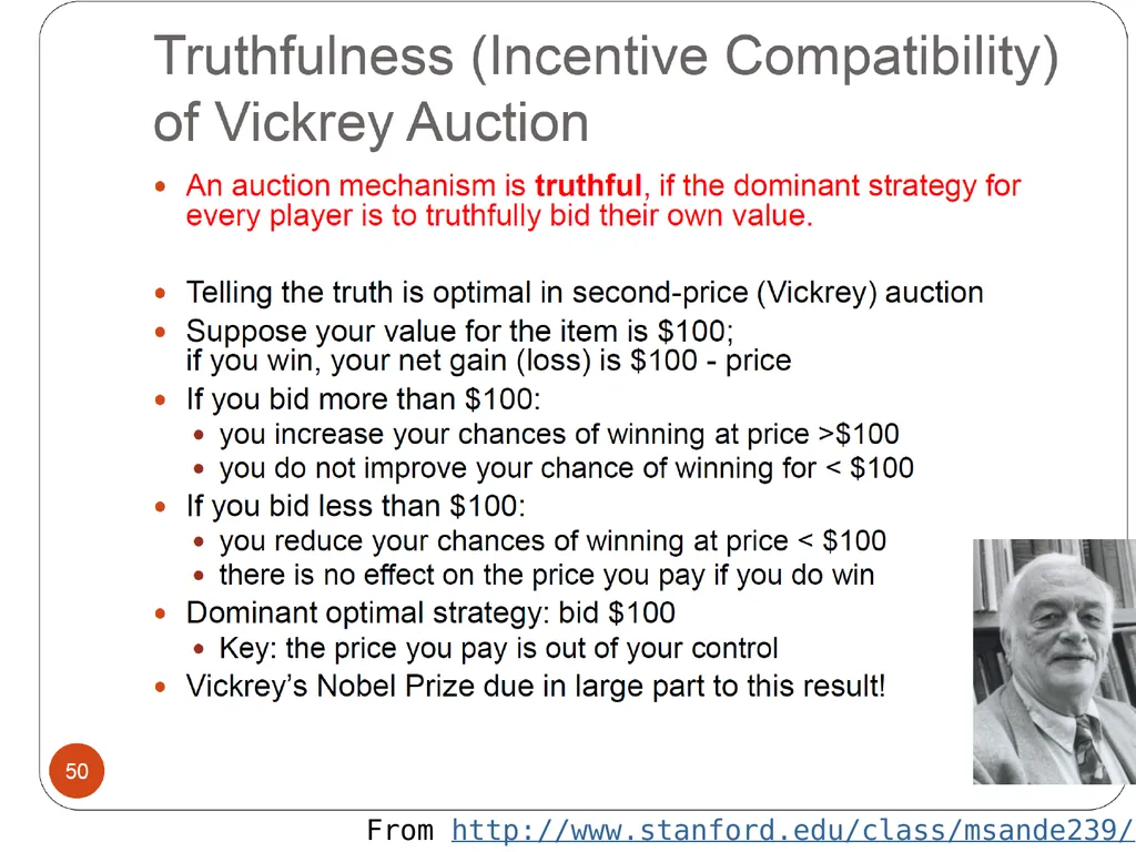
Solution: Second Price Auction (Vickery Auction)
The advertiser with the highest bid wins, but only pays the price of the second highest bid
Has the property that truthful bidding is dominant strategy [No other strategy does better] Insight: Physical auctions
Are second-price auctions!<br>
I am willing to pay 2$/click on the phrase “best asu course”
But should I be charged the full 2$ even if no one else cares for that phrase?
If I know that I will be charged my full bid price, I am likely to under-bid
I lose the auction; search engine loses revenue
Solution: Second Price Auction (Vickery Auction)
The advertiser with the highest bid wins, but only pays the price of the second highest bid
Has the property that truthful bidding is dominant strategy [No other strategy does better] Insight: Physical auctions
Are second-price auctions!<br>
34
From http://www.stanford.edu/class/msande239/<br>
35
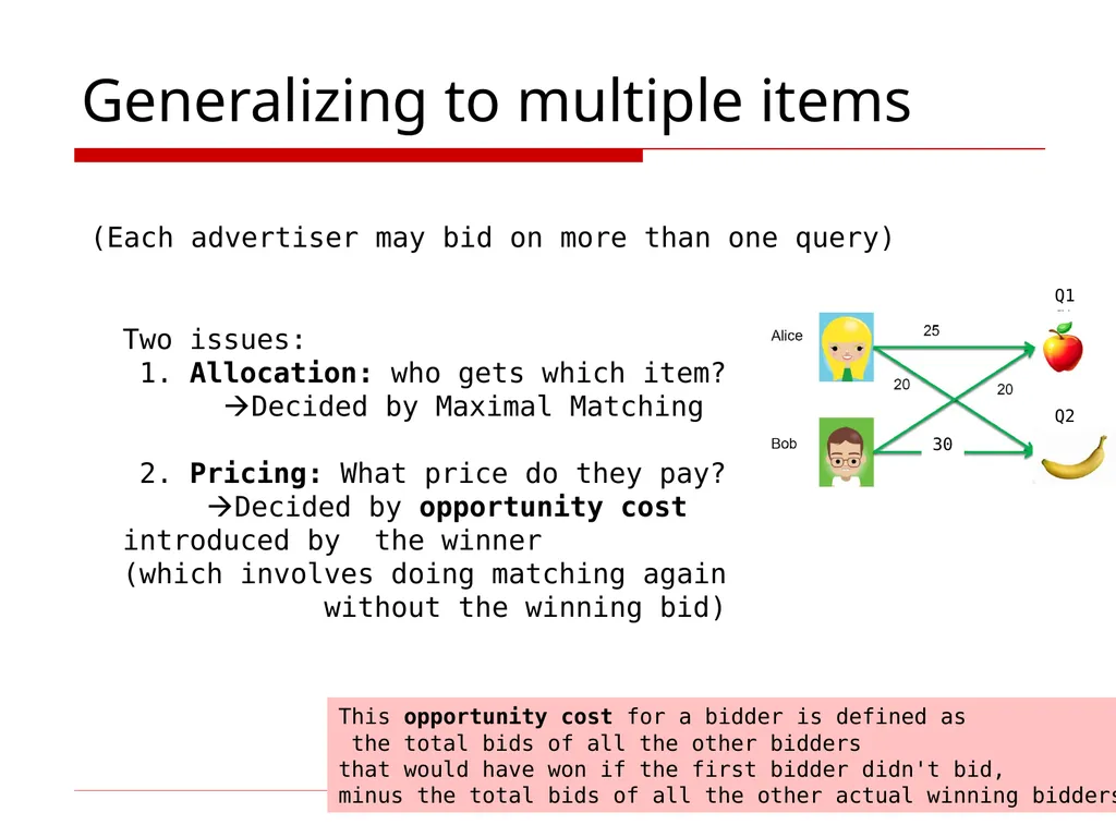
Generalizing to multiple items Two issues:
1. Allocation: who gets which item?
Decided by Maximal Matching
2. Pricing: What price do they pay?
Decided by opportunity cost introduced by the winner
(which involves doing matching again
without the winning bid) (Each advertiser may bid on more than one query) 30 Q1 Q2 This opportunity cost for a bidder is defined as
the total bids of all the other bidders
that would have won if the first bidder didn't bid,
minus the total bids of all the other actual winning bidders.<br>
1. Allocation: who gets which item?
Decided by Maximal Matching
2. Pricing: What price do they pay?
Decided by opportunity cost introduced by the winner
(which involves doing matching again
without the winning bid) (Each advertiser may bid on more than one query) 30 Q1 Q2 This opportunity cost for a bidder is defined as
the total bids of all the other bidders
that would have won if the first bidder didn't bid,
minus the total bids of all the other actual winning bidders.<br>
36
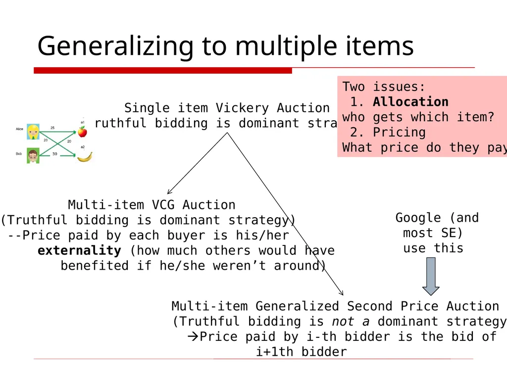
Generalizing to multiple items Single item Vickery Auction
(Truthful bidding is dominant strategy) Multi-item VCG Auction
(Truthful bidding is dominant strategy)
--Price paid by each buyer is his/her
externality (how much others would have
benefited if he/she weren’t around) Multi-item Generalized Second Price Auction
(Truthful bidding is not a dominant strategy)
Price paid by i-th bidder is the bid of
i+1th bidder Google (and
most SE)
use this Two issues:
1. Allocation
who gets which item?
2. Pricing
What price do they pay?<br>
(Truthful bidding is dominant strategy) Multi-item VCG Auction
(Truthful bidding is dominant strategy)
--Price paid by each buyer is his/her
externality (how much others would have
benefited if he/she weren’t around) Multi-item Generalized Second Price Auction
(Truthful bidding is not a dominant strategy)
Price paid by i-th bidder is the bid of
i+1th bidder Google (and
most SE)
use this Two issues:
1. Allocation
who gets which item?
2. Pricing
What price do they pay?<br>
37
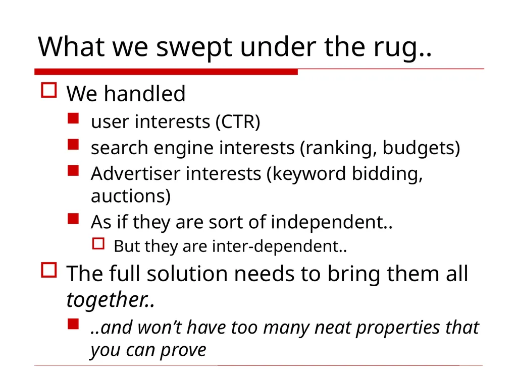
What we swept under the rug.. We handled
user interests (CTR)
search engine interests (ranking, budgets)
Advertiser interests (keyword bidding, auctions)
As if they are sort of independent..
But they are inter-dependent..
The full solution needs to bring them all together..
..and won’t have too many neat properties that you can prove<br>
user interests (CTR)
search engine interests (ranking, budgets)
Advertiser interests (keyword bidding, auctions)
As if they are sort of independent..
But they are inter-dependent..
The full solution needs to bring them all together..
..and won’t have too many neat properties that you can prove<br>
38
Ad Ranking: State of the Art Sort by
Bid Amount x Relevance We consider ads as a set, and ranking is based on user’s browsing model Sort by
Bid Amount Ads are Considered in Isolation, as both ignore Mutual influences. 38<br>
Bid Amount x Relevance We consider ads as a set, and ranking is based on user’s browsing model Sort by
Bid Amount Ads are Considered in Isolation, as both ignore Mutual influences. 38<br>
39
User’s Browsing Model User browses down staring at the first ad Abandon browsing with probability At every ad he May Process repeats for the ads below with a reduced probability Click the ad with relevance probability 39<br>
40
Mutual Influences Three Manifestations of Mutual Influences on an ad are:
Similar ads placed above
Reduces user’s residual relevance of
Relevance of other ads placed above
User may click on above ads may not view
Abandonment probability of other ads placed above
User may abandon search and may not view 40<br>
Similar ads placed above
Reduces user’s residual relevance of
Relevance of other ads placed above
User may click on above ads may not view
Abandonment probability of other ads placed above
User may abandon search and may not view 40<br>
41
Expected Profit Considering Ad Similarities Considering bids ( ), residual Relevance ( ), abandonment probability ( ), and similarities the expected profit from a set of n results is, THEOREM: Ranking maximizing expected profit considering similarities between the results is NP-Hard Proof is a reduction of independent set problem to choosing top-k ads considering similarities. Expected Profit = Even worse, constant ratio approximation algorithms are hard (unless NP = ZPP) for diversity ranking problem 41<br>
42
Dropping similarity, hence replacing Residual Relevance
( ) by Absolute Relevance ( ),
Ranking to maximize this expected utility is a sorting problem Expected Profit Considering other two Mutual Influences (2 and 3) Expected Profit = 42<br>
( ) by Absolute Relevance ( ),
Ranking to maximize this expected utility is a sorting problem Expected Profit Considering other two Mutual Influences (2 and 3) Expected Profit = 42<br>
43
Comparison to current Ad Rankings Assume abandonment probability is zero Assume
where is a constant for all ads Assumes that the user has infinite patience to go down the results until he finds the ad he wants. Assumes that abandonment probability is negatively proportional to relevance. Bid Amount x Relevance<br>
where is a constant for all ads Assumes that the user has infinite patience to go down the results until he finds the ad he wants. Assumes that abandonment probability is negatively proportional to relevance. Bid Amount x Relevance<br>
44
Generality of the Proposed Ranking The generalized ranking based on utilities. For ads utility=bid amount For documents utility=relevance Popular relevance ranking 44<br>
45
Quantifying Expected Profit Proposed strategy gives maximum profit for the entire range 45.7% 35.9% Number of Clicks
Zipf random with exponent 1.5 Abandonment probability
Uniform Random as Relevance
Uniform random as Bid Amounts
Uniform random Difference in profit between RF and competing strategy is significant 45<br>
Zipf random with exponent 1.5 Abandonment probability
Uniform Random as Relevance
Uniform random as Bid Amounts
Uniform random Difference in profit between RF and competing strategy is significant 45<br>
46
Optimal Ad-Ranking for Profit Maximization.
Raju Balakrishnan, Subbarao Kabmbhampati. WebDB 2008
Yahoo! Research Key scientific Challenge award for Computation advertising, 2009-10 Publication and Recognition 46<br>
Raju Balakrishnan, Subbarao Kabmbhampati. WebDB 2008
Yahoo! Research Key scientific Challenge award for Computation advertising, 2009-10 Publication and Recognition 46<br>
47
Online algorithms Classic model of algorithms
You get to see the entire input, then compute some function of it
In this context, “offline algorithm”
Online algorithm
You get to see the input one piece at a time, and need to make irrevocable decisions along the way
Similar to data stream models<br>
You get to see the entire input, then compute some function of it
In this context, “offline algorithm”
Online algorithm
You get to see the input one piece at a time, and need to make irrevocable decisions along the way
Similar to data stream models<br>
48
Example: Bipartite matching 1 2 3 4 a b c d Girls Boys<br>
49
Example: Bipartite matching 1 2 3 4 a b c d M = {(1,a),(2,b),(3,d)} is a matching
Cardinality of matching = |M| = 3 Girls Boys<br>
Cardinality of matching = |M| = 3 Girls Boys<br>
50
Example: Bipartite matching 1 2 3 4 a b c d Girls Boys M = {(1,c),(2,b),(3,d),(4,a)} is a
perfect matching<br>
perfect matching<br>
51
Matching Algorithm Problem: Find a maximum-cardinality matching for a given bipartite graph
A perfect one if it exists
There is a polynomial-time offline algorithm (Hopcroft and Karp 1973)
But what if we don’t have the entire graph upfront?<br>
A perfect one if it exists
There is a polynomial-time offline algorithm (Hopcroft and Karp 1973)
But what if we don’t have the entire graph upfront?<br>
52
Online problem Initially, we are given the set Boys
In each round, one girl’s choices are revealed
At that time, we have to decide to either:
Pair the girl with a boy
Don’t pair the girl with any boy
Example of application: assigning tasks to servers<br>
In each round, one girl’s choices are revealed
At that time, we have to decide to either:
Pair the girl with a boy
Don’t pair the girl with any boy
Example of application: assigning tasks to servers<br>
53
Online problem 1 2 3 4 (1,a) (2,b) (3,d)<br>
54
Greedy algorithm Pair the new girl with any eligible boy
If there is none, don’t pair girl
How good is the algorithm?<br>
If there is none, don’t pair girl
How good is the algorithm?<br>
55
Competitive Ratio For input I, suppose greedy produces matching Mgreedy while an optimal matching is Mopt
Competitive ratio =
minall possible inputs I (|Mgreedy|/|Mopt|)<br>
Competitive ratio =
minall possible inputs I (|Mgreedy|/|Mopt|)<br>
56
Analyzing the greedy algorithm Consider the set G of girls matched in Mopt but not in Mgreedy
Then it must be the case that every boy adjacent to girls in G is already matched in Mgreedy
There must be at least |G| such boys
Otherwise the optimal algorithm could not have matched all the G girls
Therefore
|Mgreedy| ¸ |G| = |Mopt - Mgreedy|
|Mgreedy|/|Mopt| ¸ 1/2<br>
Then it must be the case that every boy adjacent to girls in G is already matched in Mgreedy
There must be at least |G| such boys
Otherwise the optimal algorithm could not have matched all the G girls
Therefore
|Mgreedy| ¸ |G| = |Mopt - Mgreedy|
|Mgreedy|/|Mopt| ¸ 1/2<br>
57
Worst-case scenario 1 2 3 4 (1,a) (2,b)<br>