Search Engines Information Retrieval in Practice

slide1. Search Engines Information Retrieval in Practice All slides ©Addison Wesley, 2008 TexPoint fonts used in EMF.
Read the TexPoint manual before you delete this box.: AA<br>
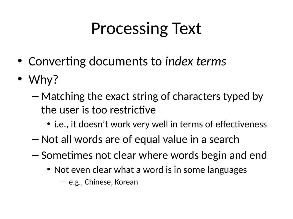
slide2. Processing Text Converting documents to index terms
Why?
Matching the exact string of characters typed by the user is too restrictive
i.e., it doesn’t work very well in terms of effectiveness
Not all words are of equal value in a search
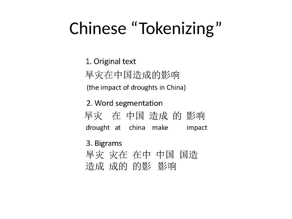
Sometimes not clear where words begin and end
Not even clear what a word is in some languages
e.g., Chinese, Korean<br>
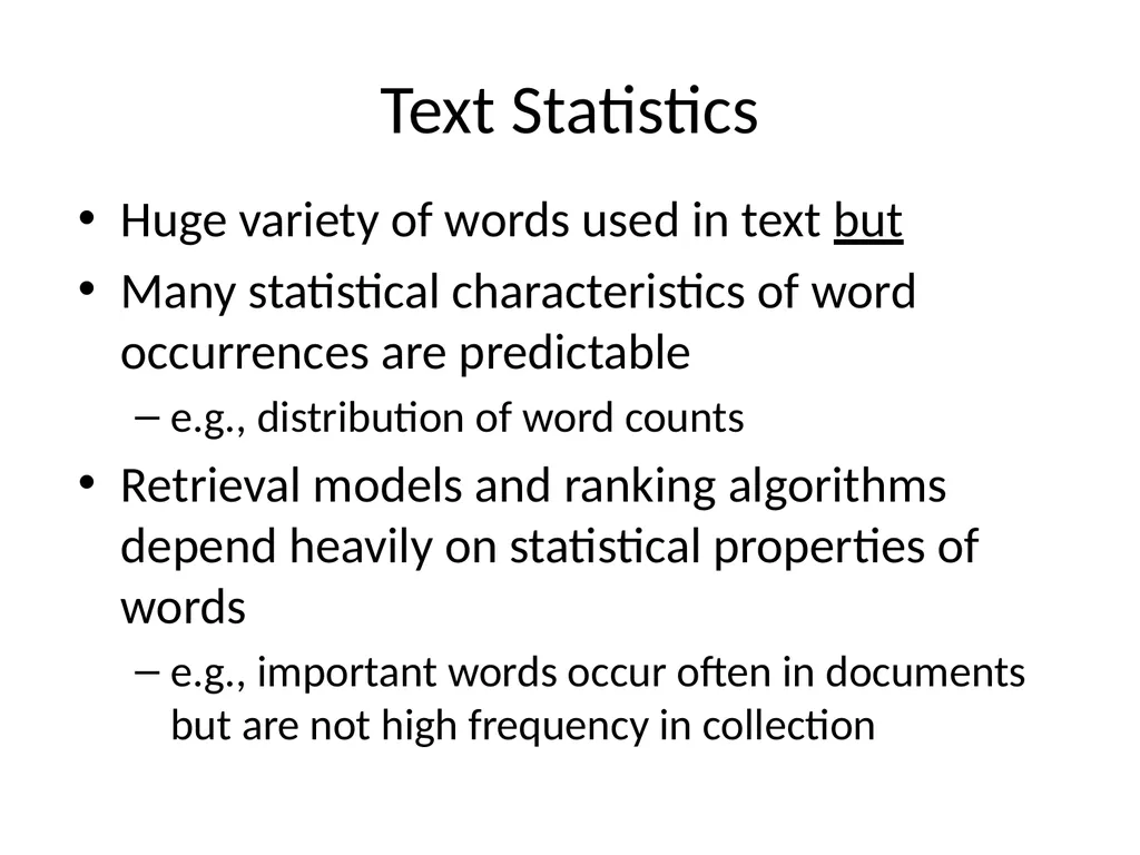
slide3. Text Statistics Huge variety of words used in text but
Many statistical characteristics of word occurrences are predictable
e.g., distribution of word counts
Retrieval models and ranking algorithms depend heavily on statistical properties of words
e.g., important words occur often in documents but are not high frequency in collection<br>
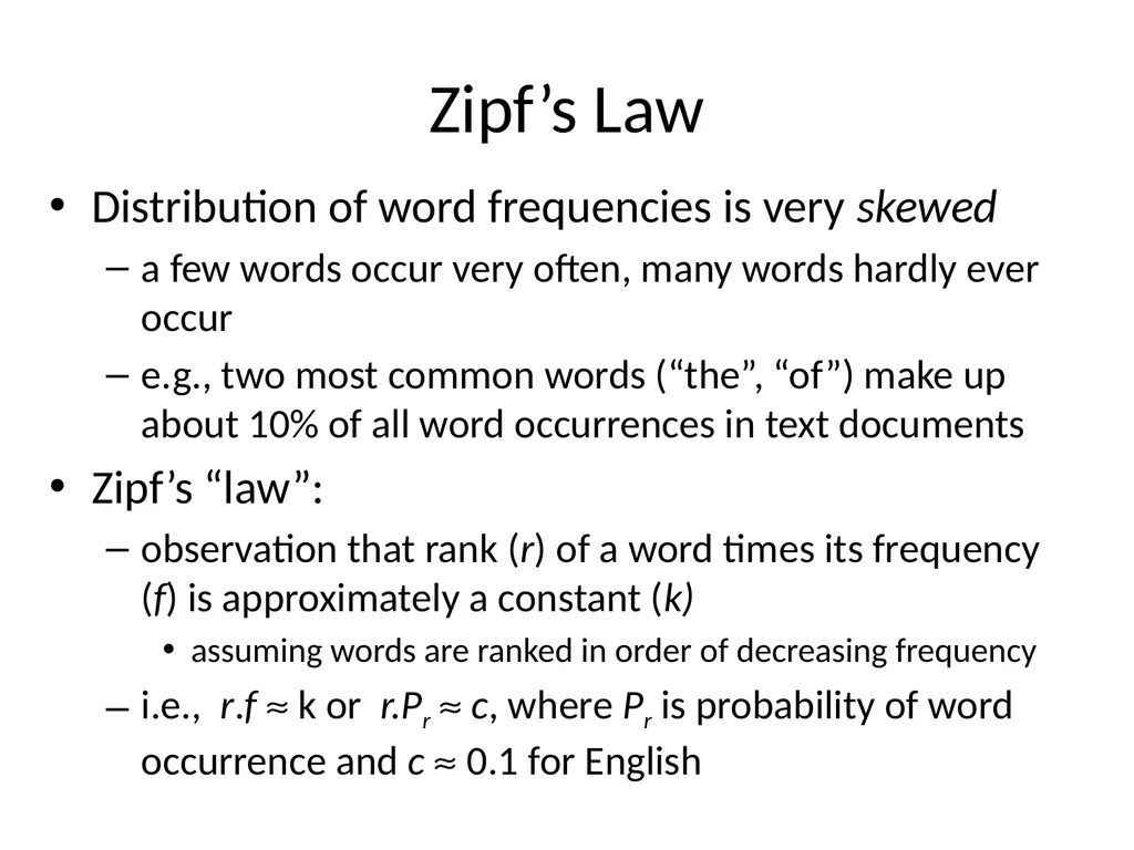
slide4. Zipf’s Law Distribution of word frequencies is very skewed
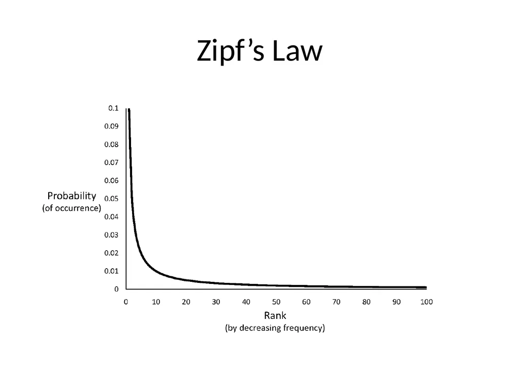
a few words occur very often, many words hardly ever occur
e.g., two most common words (“the”, “of”) make up about 10% of all word occurrences in text documents
Zipf’s “law”:
observation that rank (r) of a word times its frequency (f) is approximately a constant (k)
assuming words are ranked in order of decreasing frequency
i.e., r.f » k or r.Pr » c, where Pr is probability of word occurrence and c » 0.1 for English<br>
slide5. Zipf’s Law<br>
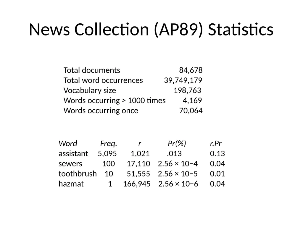
slide6. News Collection (AP89) Statistics Total documents 84,678
Total word occurrences 39,749,179
Vocabulary size 198,763
Words occurring > 1000 times 4,169
Words occurring once 70,064 Word Freq. r Pr(%) r.Pr
assistant 5,095 1,021 .013 0.13
sewers 100 17,110 2.56 × 10−4 0.04
toothbrush 10 51,555 2.56 × 10−5 0.01
hazmat 1 166,945 2.56 × 10−6 0.04<br>
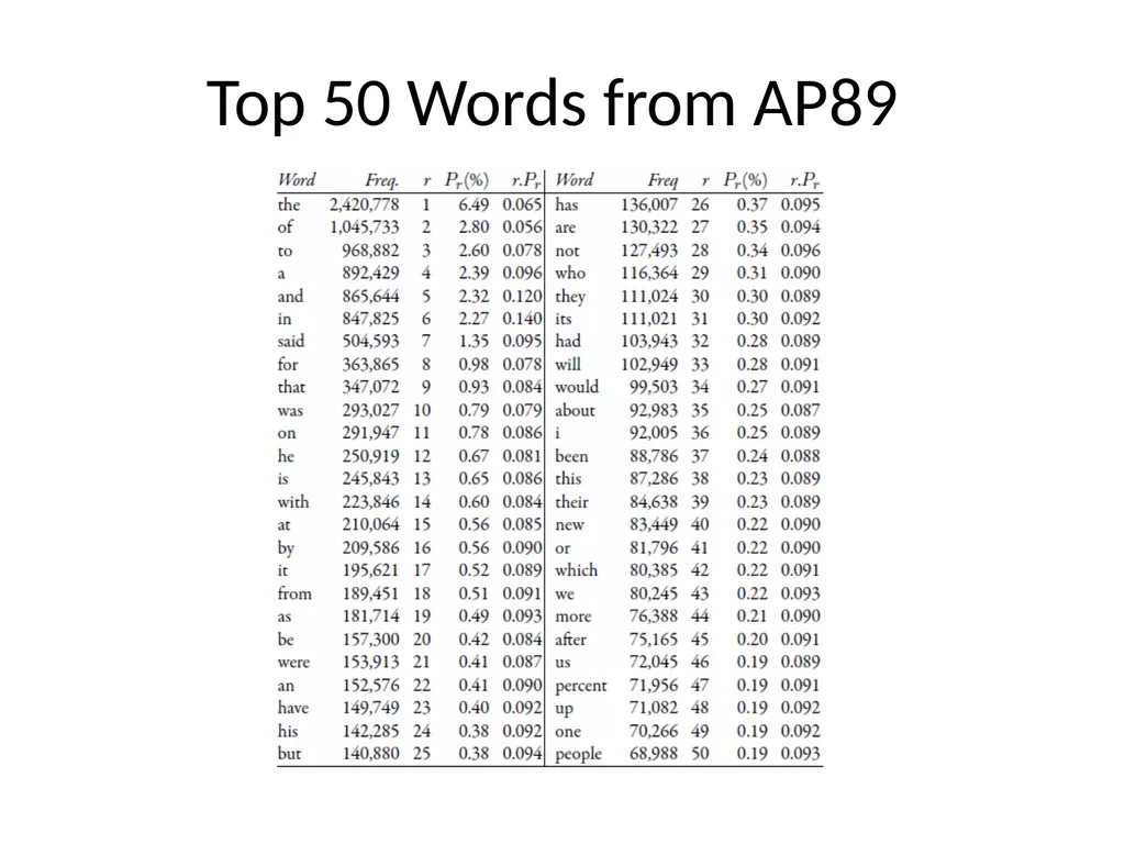
slide7. Top 50 Words from AP89<br>
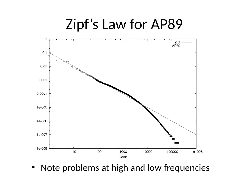
slide8. Zipf’s Law for AP89 Note problems at high and low frequencies<br>
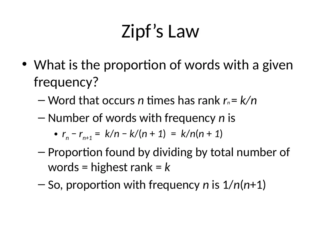
slide9. Zipf’s Law What is the proportion of words with a given frequency?
Word that occurs n times has rank rn = k/n
Number of words with frequency n is
rn − rn+1 = k/n − k/(n + 1) = k/n(n + 1)
Proportion found by dividing by total number of words = highest rank = k
So, proportion with frequency n is 1/n(n+1)<br>
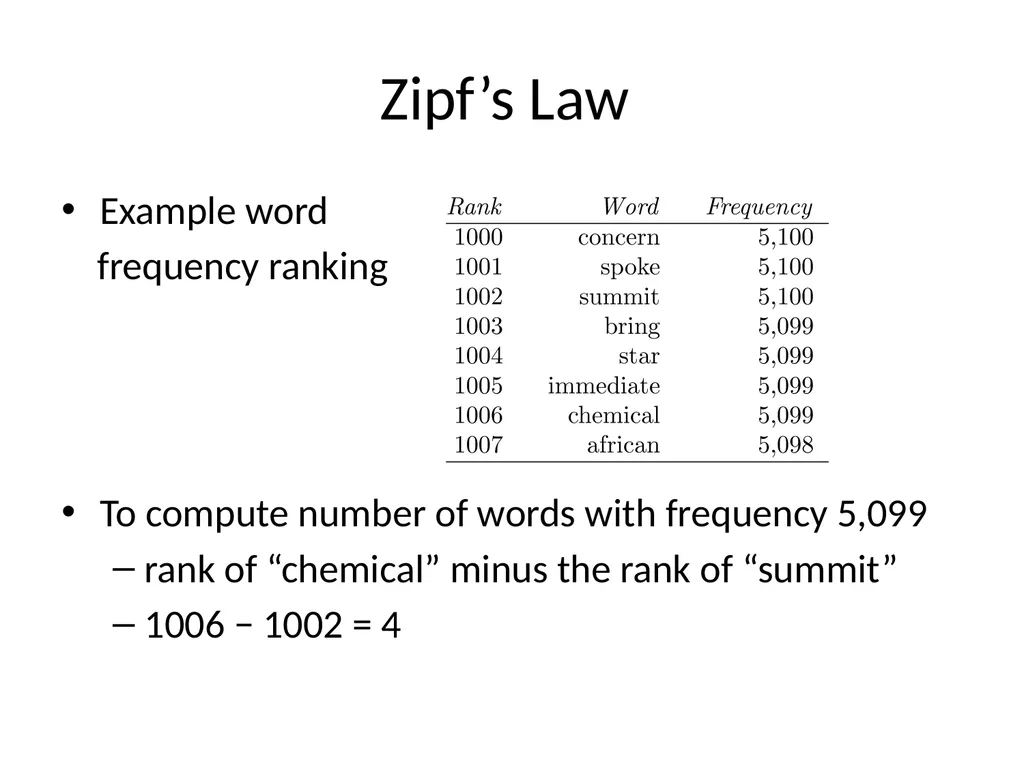
slide10. Zipf’s Law Example word
frequency ranking

To compute number of words with frequency 5,099
rank of “chemical” minus the rank of “summit”
1006 − 1002 = 4<br>
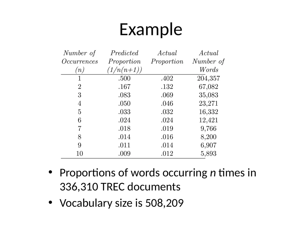
slide11. Example Proportions of words occurring n times in 336,310 TREC documents
Vocabulary size is 508,209<br>
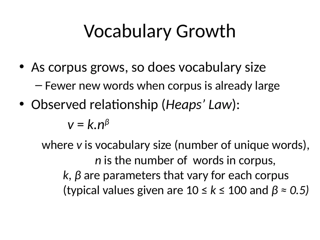
slide12. Vocabulary Growth As corpus grows, so does vocabulary size
Fewer new words when corpus is already large
Observed relationship (Heaps’ Law):
v = k.nβ
where v is vocabulary size (number of unique words), n is the number of words in corpus, k, β are parameters that vary for each corpus (typical values given are 10 ≤ k ≤ 100 and β ≈ 0.5)<br>
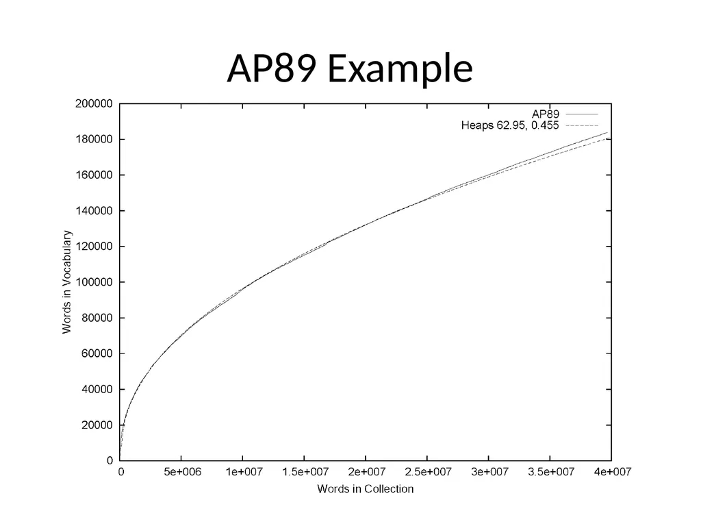
slide13. AP89 Example<br>
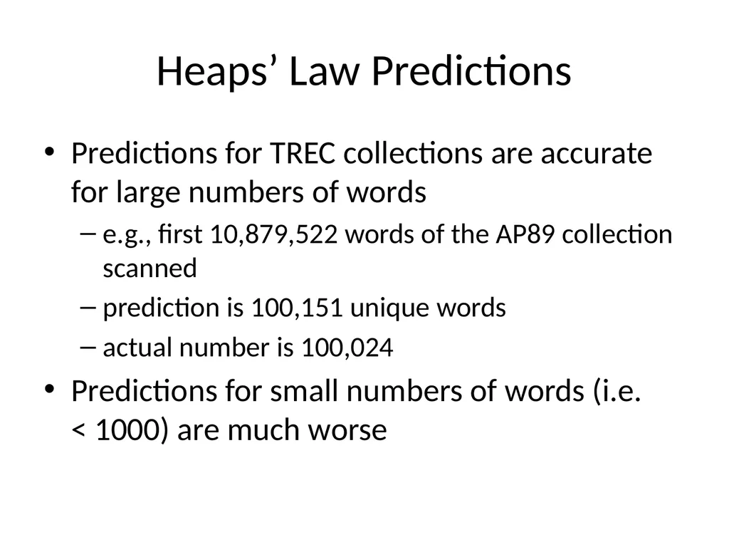
slide14. Heaps’ Law Predictions Predictions for TREC collections are accurate for large numbers of words
e.g., first 10,879,522 words of the AP89 collection scanned
prediction is 100,151 unique words
actual number is 100,024
Predictions for small numbers of words (i.e. < 1000) are much worse<br>
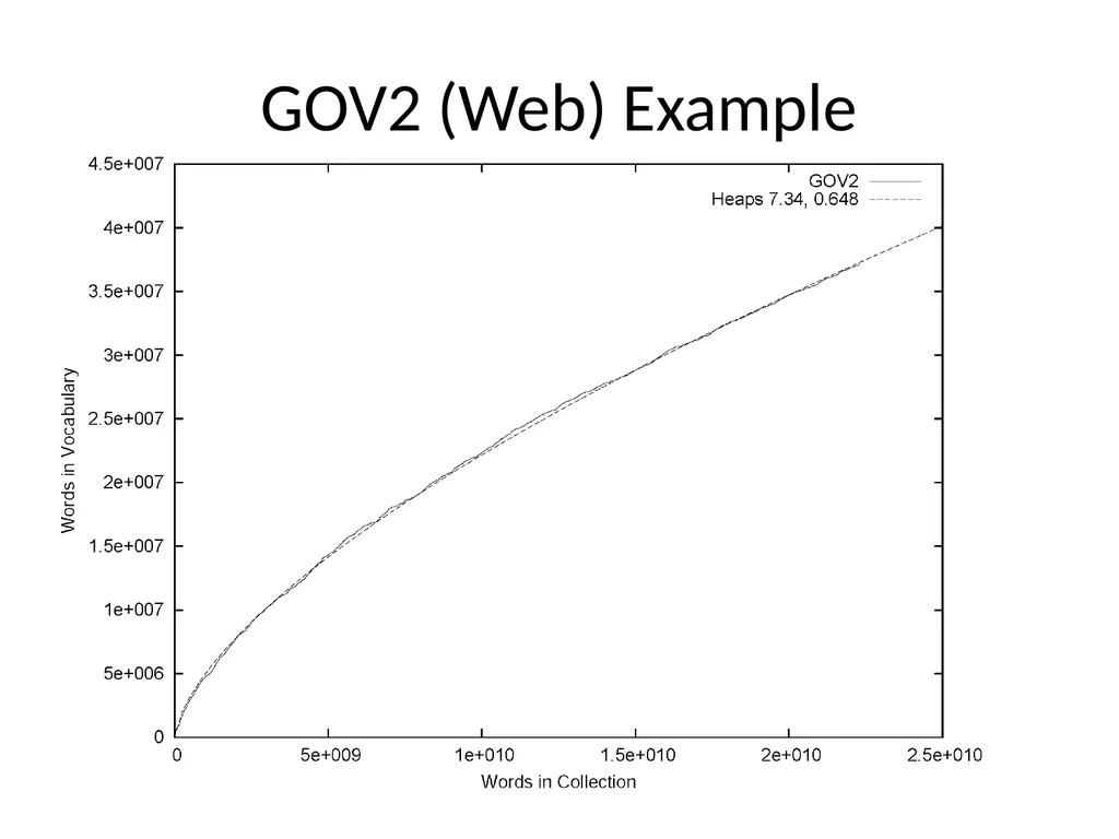
slide15. GOV2 (Web) Example<br>
slide16. Web Example Heaps’ Law works with very large corpora
new words occurring even after seeing 30 million!
parameter values different than typical TREC values
New words come from a variety of sources
spelling errors, invented words (e.g. product, company names), code, other languages, email addresses, etc.
Search engines must deal with these large and growing vocabularies<br>
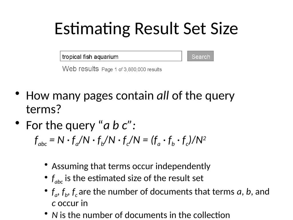
slide17. Estimating Result Set Size How many pages contain all of the query terms?
For the query “a b c”:
fabc = N · fa/N · fb/N · fc/N = (fa · fb · fc)/N2

Assuming that terms occur independently
fabc is the estimated size of the result set
fa, fb, fc are the number of documents that terms a, b, and c occur in
N is the number of documents in the collection<br>
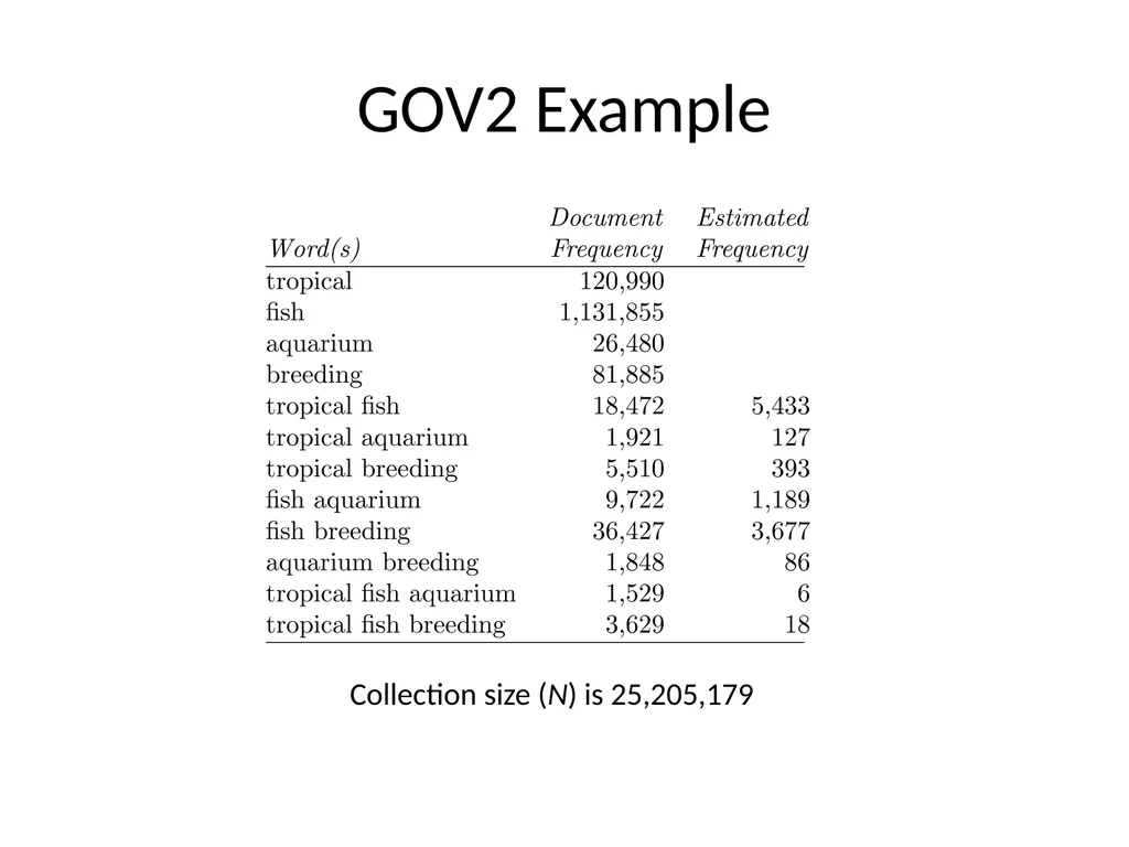
slide18. GOV2 Example Collection size (N) is 25,205,179<br>
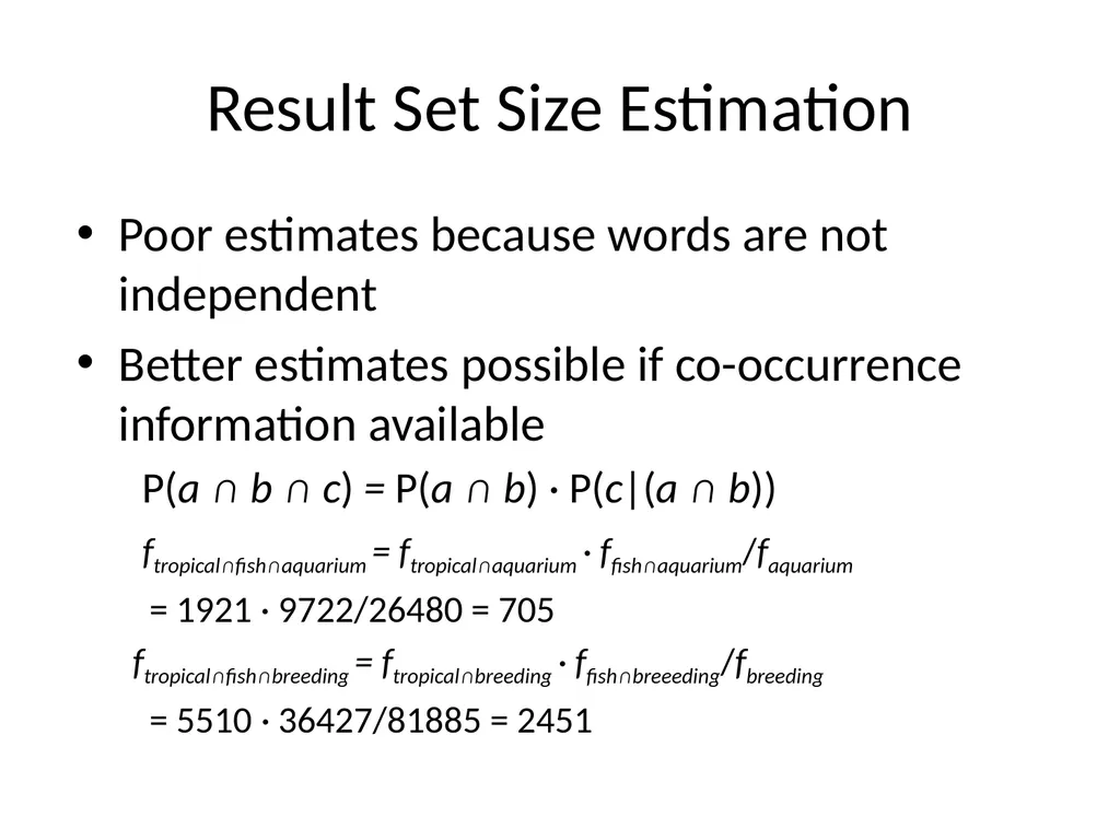
slide19. Result Set Size Estimation Poor estimates because words are not independent
Better estimates possible if co-occurrence information available
P(a ∩ b ∩ c) = P(a ∩ b) · P(c|(a ∩ b))
ftropical∩fish∩aquarium = ftropical∩aquarium · ffish∩aquarium/faquarium
= 1921 · 9722/26480 = 705
ftropical∩fish∩breeding = ftropical∩breeding · ffish∩breeeding/fbreeding
= 5510 · 36427/81885 = 2451<br>
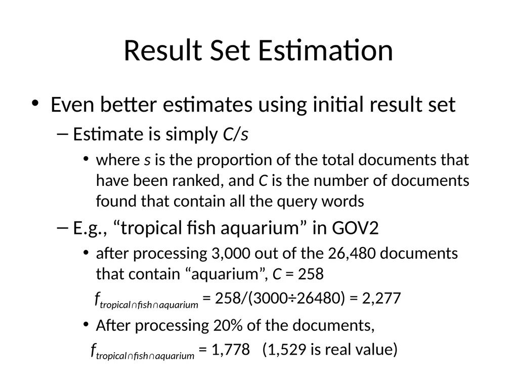
slide20. Result Set Estimation Even better estimates using initial result set
Estimate is simply C/s
where s is the proportion of the total documents that have been ranked, and C is the number of documents found that contain all the query words
E.g., “tropical fish aquarium” in GOV2
after processing 3,000 out of the 26,480 documents that contain “aquarium”, C = 258
ftropical∩fish∩aquarium = 258/(3000÷26480) = 2,277
After processing 20% of the documents,
ftropical∩fish∩aquarium = 1,778 (1,529 is real value)<br>
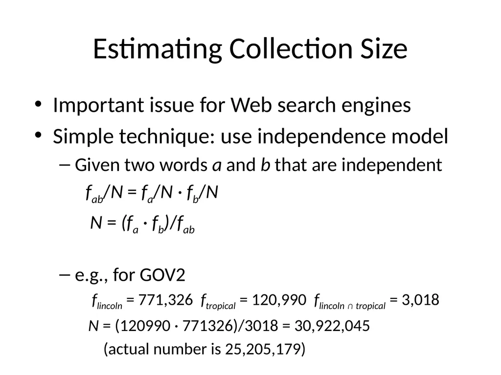
slide21. Estimating Collection Size Important issue for Web search engines
Simple technique: use independence model
Given two words a and b that are independent
fab/N = fa/N · fb/N
N = (fa · fb)/fab

e.g., for GOV2
flincoln = 771,326 ftropical = 120,990 flincoln ∩ tropical = 3,018
N = (120990 · 771326)/3018 = 30,922,045
(actual number is 25,205,179)<br>
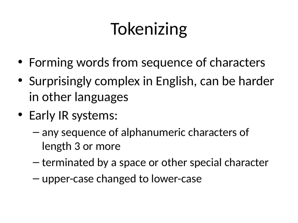
slide22. Tokenizing Forming words from sequence of characters
Surprisingly complex in English, can be harder in other languages
Early IR systems:
any sequence of alphanumeric characters of length 3 or more
terminated by a space or other special character
upper-case changed to lower-case<br>
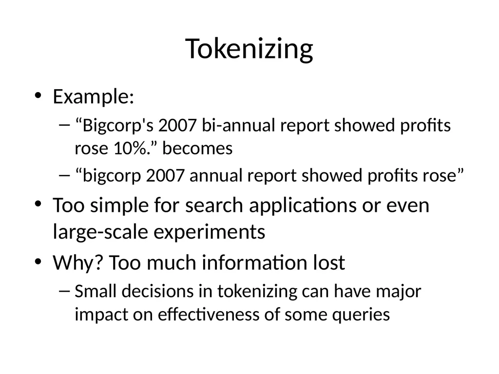
slide23. Tokenizing Example:
“Bigcorp's 2007 bi-annual report showed profits rose 10%.” becomes
“bigcorp 2007 annual report showed profits rose”
Too simple for search applications or even large-scale experiments
Why? Too much information lost
Small decisions in tokenizing can have major impact on effectiveness of some queries<br>
slide24. Tokenizing Problems Small words can be important in some queries, usually in combinations
xp, ma, pm, ben e king, el paso, master p, gm, j lo, world war II
Both hyphenated and non-hyphenated forms of many words are common
Sometimes hyphen is not needed
e-bay, wal-mart, active-x, cd-rom, t-shirts
At other times, hyphens should be considered either as part of the word or a word separator
winston-salem, mazda rx-7, e-cards, pre-diabetes, t-mobile, spanish-speaking<br>
slide25. Tokenizing Problems Special characters are an important part of tags, URLs, code in documents
Capitalized words can have different meaning from lower case words
Bush, Apple
Apostrophes can be a part of a word, a part of a possessive, or just a mistake
rosie o'donnell, can't, don't, 80's, 1890's, men's straw hats, master's degree, england's ten largest cities, shriner's<br>
slide26. Tokenizing Problems Numbers can be important, including decimals
nokia 3250, top 10 courses, united 93, quicktime 6.5 pro, 92.3 the beat, 288358
Periods can occur in numbers, abbreviations, URLs, ends of sentences, and other situations
I.B.M., Ph.D., cs.umass.edu, F.E.A.R.
Note: tokenizing steps for queries must be identical to steps for documents<br>
slide27. Tokenizing Process First step is to use parser to identify appropriate parts of document to tokenize
Defer complex decisions to other components
word is any sequence of alphanumeric characters, terminated by a space or special character, with everything converted to lower-case
everything indexed
example: 92.3 → 92 3 but search finds documents with 92 and 3 adjacent
incorporate some rules to reduce dependence on query transformation components<br>
slide28. Tokenizing Process Not that different than simple tokenizing process used in past
Examples of rules used with TREC
Apostrophes in words ignored
o’connor → oconnor bob’s → bobs
Periods in abbreviations ignored
I.B.M. → ibm Ph.D. → ph d<br>
slide29. Stopping Function words (determiners, prepositions) have little meaning on their own
High occurrence frequencies
Treated as stopwords (i.e. removed)
reduce index space, improve response time, improve effectiveness
Can be important in combinations
e.g., “to be or not to be”<br>
slide30. Stopping Stopword list can be created from high-frequency words or based on a standard list
Lists are customized for applications, domains, and even parts of documents
e.g., “click” is a good stopword for anchor text
Best policy is to index all words in documents, make decisions about which words to use at query time<br>
slide31. Stemming Many morphological variations of words
inflectional (plurals, tenses)
derivational (making verbs nouns etc.)
In most cases, these have the same or very similar meanings
Stemmers attempt to reduce morphological variations of words to a common stem
usually involves removing suffixes
Can be done at indexing time or as part of query processing (like stopwords)<br>
slide32. Stemming Generally a small but significant effectiveness improvement
can be crucial for some languages
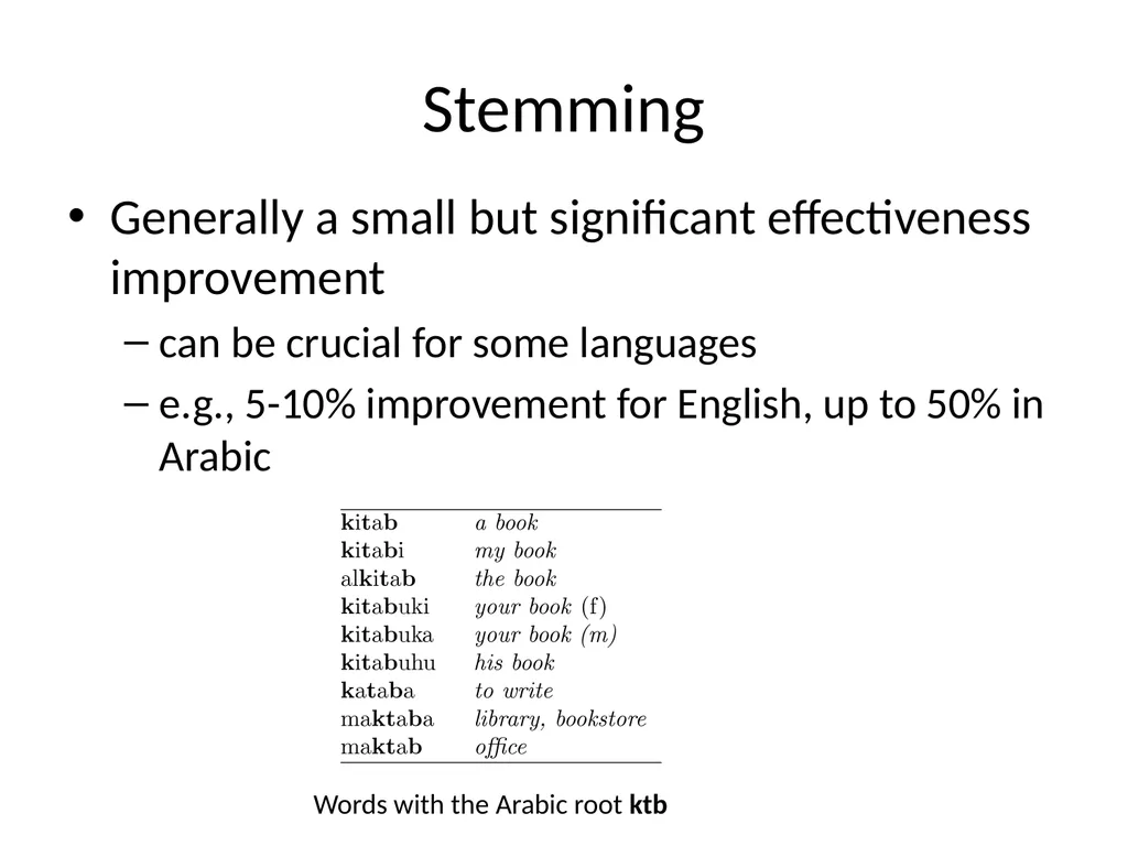
e.g., 5-10% improvement for English, up to 50% in Arabic Words with the Arabic root ktb<br>
slide33. Stemming Two basic types
Dictionary-based: uses lists of related words
Algorithmic: uses program to determine related words
Algorithmic stemmers
suffix-s: remove ‘s’ endings assuming plural
e.g., cats → cat, lakes → lake, wiis → wii
Many false negatives: supplies → supplie
Some false positives: ups → up<br>
slide34. Porter Stemmer Algorithmic stemmer used in IR experiments since the 70s
Consists of a series of rules designed to the longest possible suffix at each step
Effective in TREC
Produces stems not words
Makes a number of errors and difficult to modify<br>
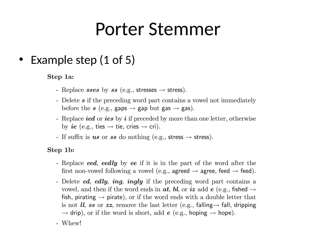
slide35. Porter Stemmer Example step (1 of 5)<br>
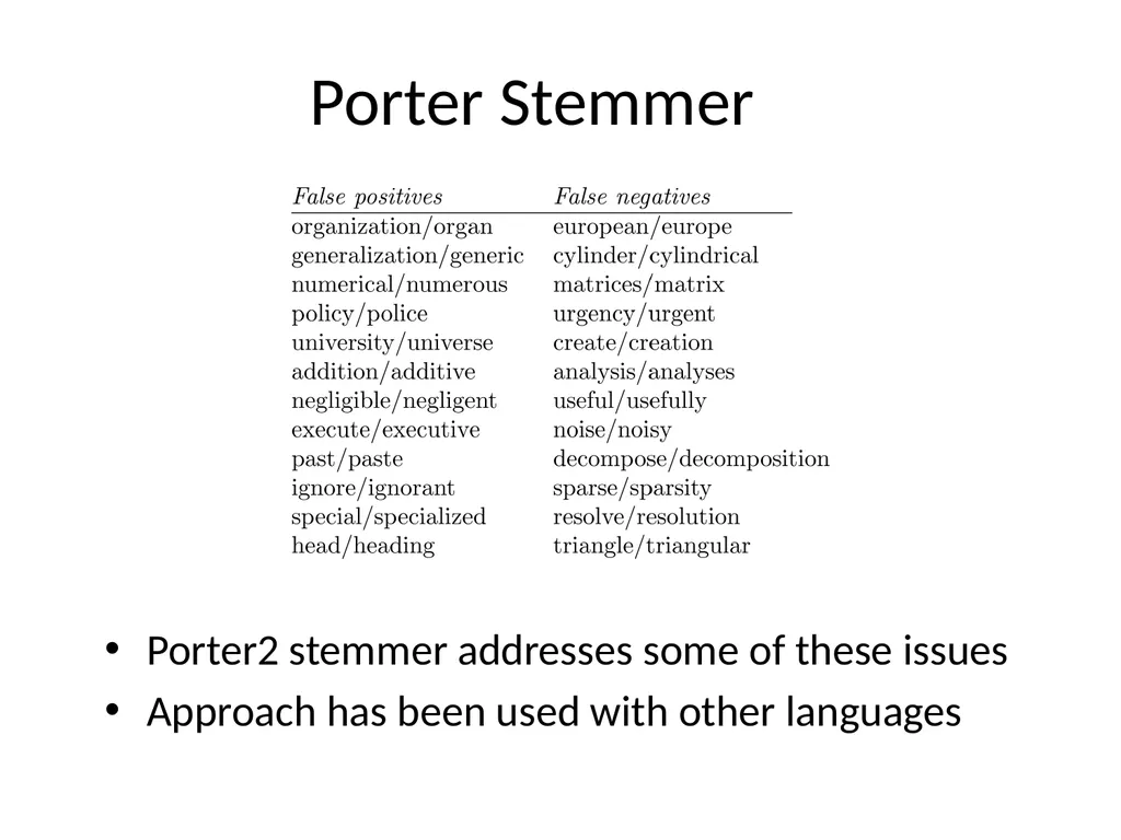
slide36. Porter Stemmer Porter2 stemmer addresses some of these issues
Approach has been used with other languages<br>
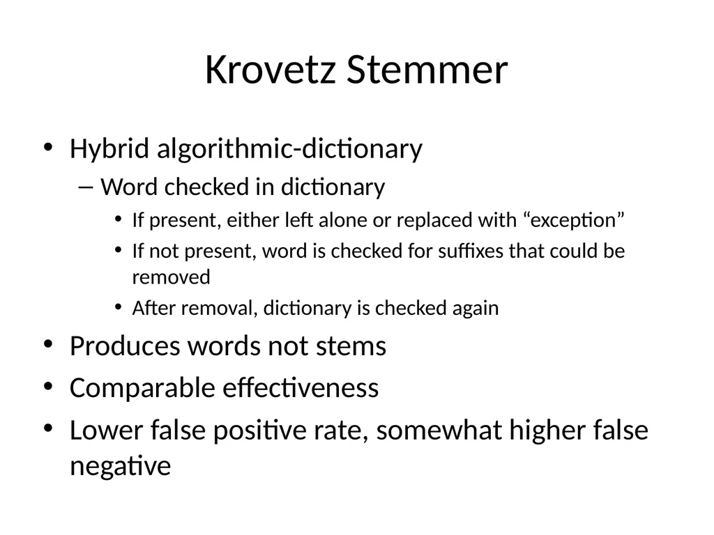
slide37. Krovetz Stemmer Hybrid algorithmic-dictionary
Word checked in dictionary
If present, either left alone or replaced with “exception”
If not present, word is checked for suffixes that could be removed
After removal, dictionary is checked again
Produces words not stems
Comparable effectiveness
Lower false positive rate, somewhat higher false negative<br>
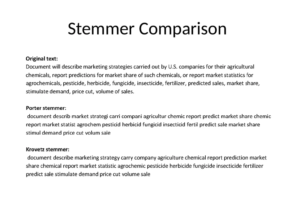
slide38. Stemmer Comparison<br>
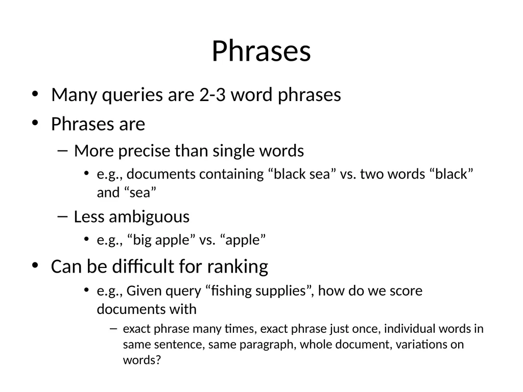
slide39. Phrases Many queries are 2-3 word phrases
Phrases are
More precise than single words
e.g., documents containing “black sea” vs. two words “black” and “sea”
Less ambiguous
e.g., “big apple” vs. “apple”
Can be difficult for ranking
e.g., Given query “fishing supplies”, how do we score documents with
exact phrase many times, exact phrase just once, individual words in same sentence, same paragraph, whole document, variations on words?<br>
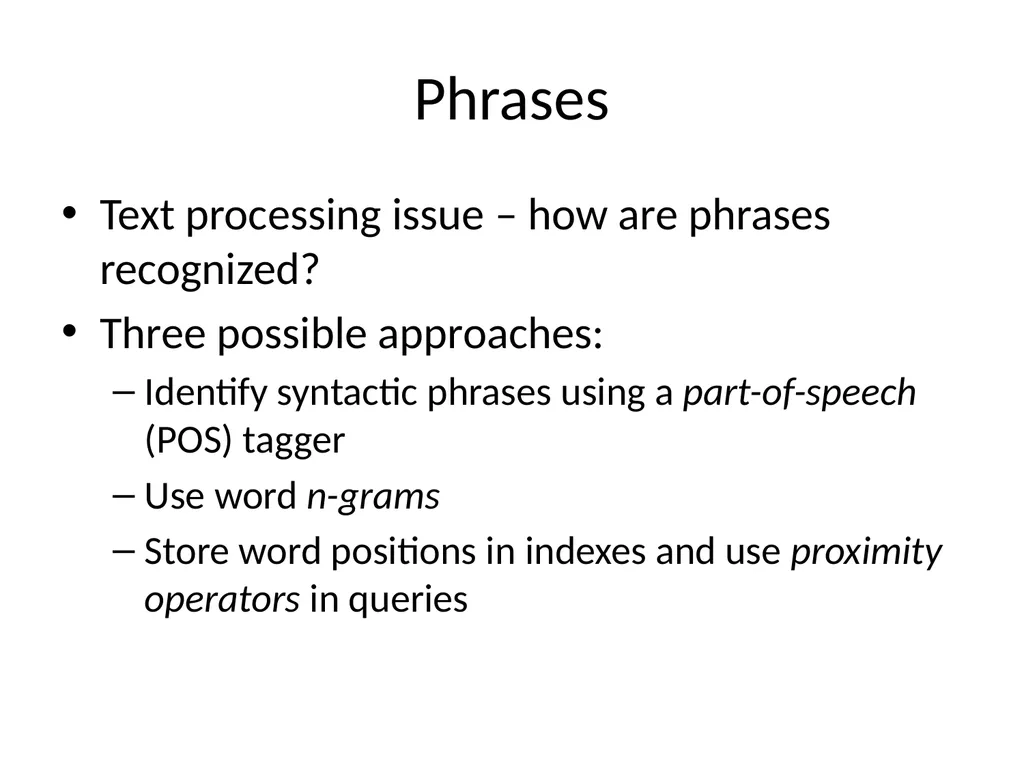
slide40. Phrases Text processing issue – how are phrases recognized?
Three possible approaches:
Identify syntactic phrases using a part-of-speech (POS) tagger
Use word n-grams
Store word positions in indexes and use proximity operators in queries<br>
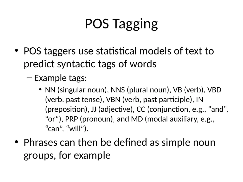
slide41. POS Tagging POS taggers use statistical models of text to predict syntactic tags of words
Example tags:
NN (singular noun), NNS (plural noun), VB (verb), VBD (verb, past tense), VBN (verb, past participle), IN (preposition), JJ (adjective), CC (conjunction, e.g., “and”, “or”), PRP (pronoun), and MD (modal auxiliary, e.g., “can”, “will”).
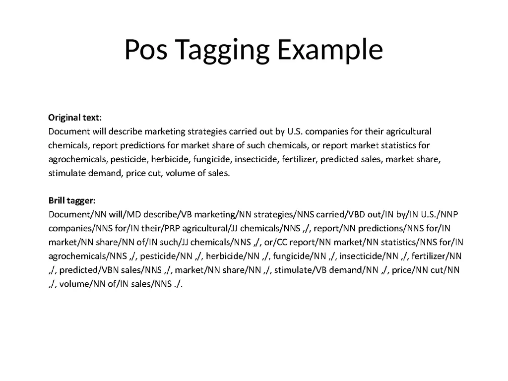
Phrases can then be defined as simple noun groups, for example<br>
slide42. Pos Tagging Example<br>
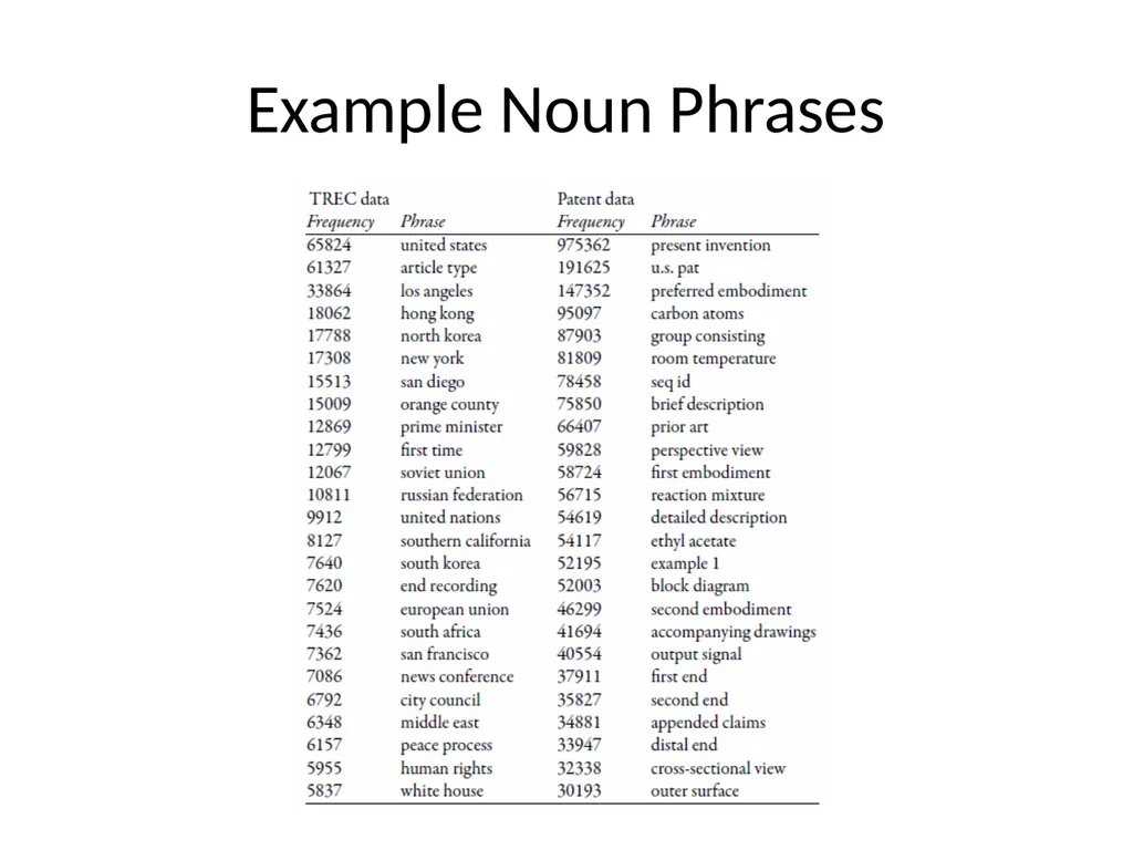
slide43. Example Noun Phrases<br>
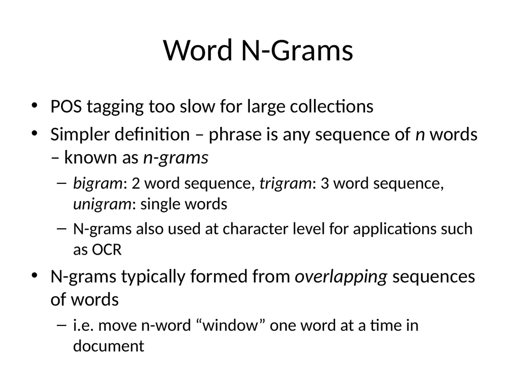
slide44. Word N-Grams POS tagging too slow for large collections
Simpler definition – phrase is any sequence of n words – known as n-grams
bigram: 2 word sequence, trigram: 3 word sequence, unigram: single words
N-grams also used at character level for applications such as OCR
N-grams typically formed from overlapping sequences of words
i.e. move n-word “window” one word at a time in document<br>
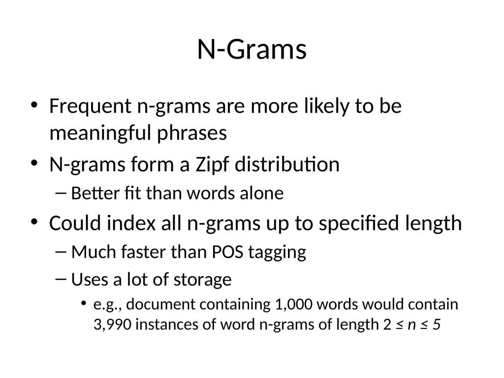
slide45. N-Grams Frequent n-grams are more likely to be meaningful phrases
N-grams form a Zipf distribution
Better fit than words alone
Could index all n-grams up to specified length
Much faster than POS tagging
Uses a lot of storage
e.g., document containing 1,000 words would contain 3,990 instances of word n-grams of length 2 ≤ n ≤ 5<br>
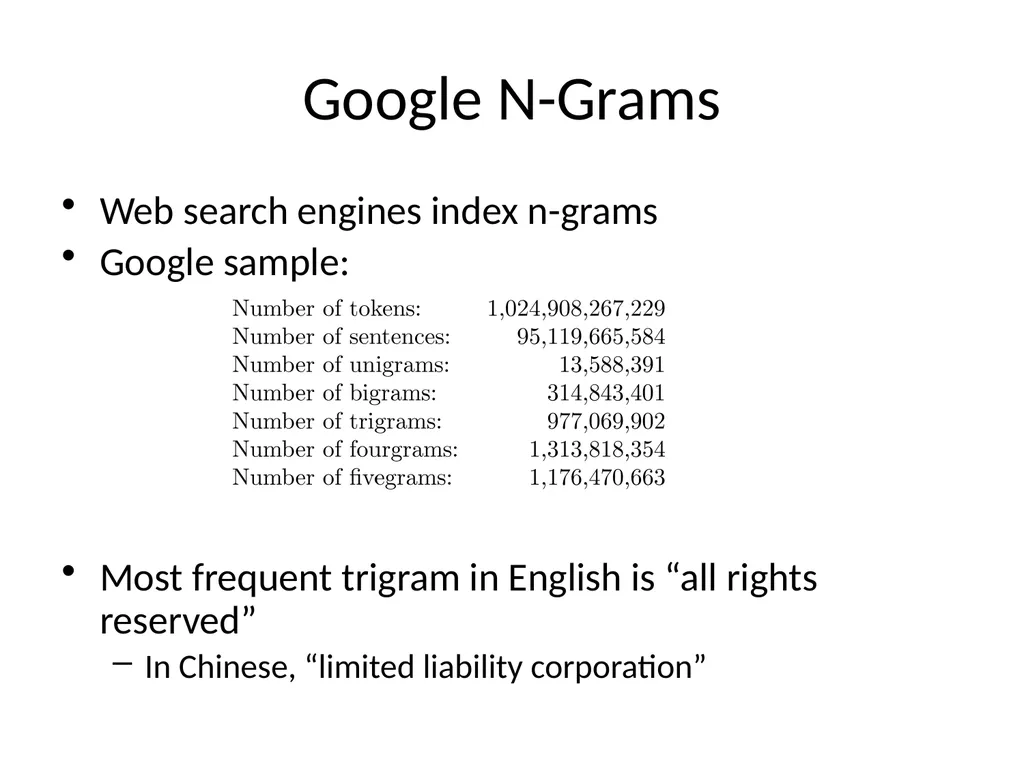
slide46. Google N-Grams Web search engines index n-grams
Google sample:

Most frequent trigram in English is “all rights reserved”
In Chinese, “limited liability corporation”<br>
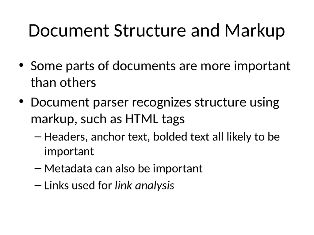
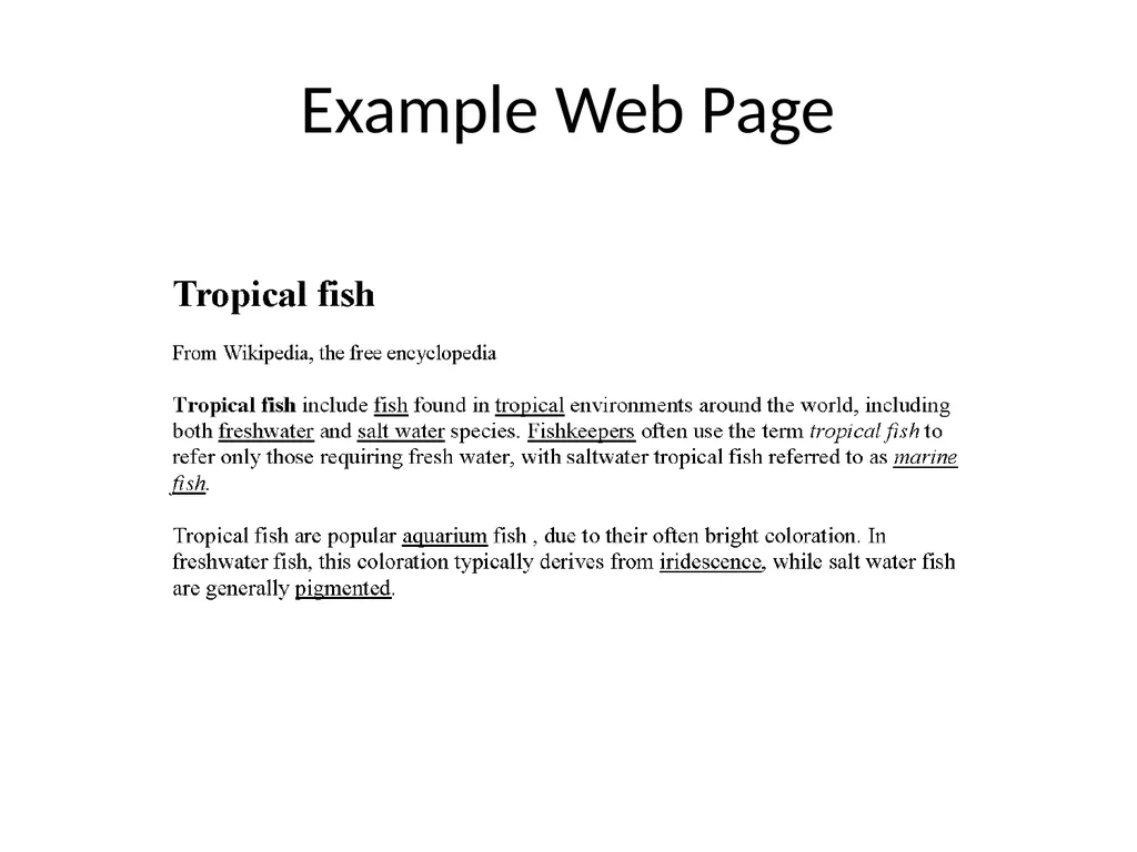
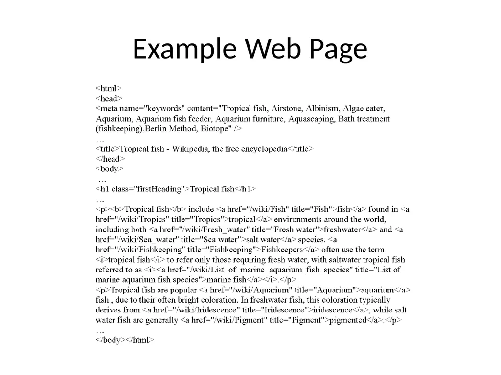
slide47. Document Structure and Markup Some parts of documents are more important than others
Document parser recognizes structure using markup, such as HTML tags
Headers, anchor text, bolded text all likely to be important
Metadata can also be important
Links used for link analysis<br>
slide48. Example Web Page<br>
slide49. Example Web Page<br>
slide50. Link Analysis Links are a key component of the Web
Important for navigation, but also for search
e.g., <a href="http://example.com" >Example website</a>
“Example website” is the anchor text
“http://example.com” is the destination link
both are used by search engines<br>
slide51. Anchor Text Used as a description of the content of the destination page
i.e., collection of anchor text in all links pointing to a page used as an additional text field
Anchor text tends to be short, descriptive, and similar to query text
Retrieval experiments have shown that anchor text has significant impact on effectiveness for some types of queries
i.e., more than PageRank<br>
slide52. PageRank Billions of web pages, some more informative than others
Links can be viewed as information about the popularity (authority?) of a web page
can be used by ranking algorithm
Inlink count could be used as simple measure
Link analysis algorithms like PageRank provide more reliable ratings
less susceptible to link spam<br>
slide53. Random Surfer Model Browse the Web using the following algorithm:
Choose a random number r between 0 and 1
If r < λ:
Go to a random page
If r ≥ λ:
Click a link at random on the current page
Start again
PageRank of a page is the probability that the “random surfer” will be looking at that page
links from popular pages will increase PageRank of pages they point to<br>
slide54. Dangling Links Random jump prevents getting stuck on pages that
do not have links
contains only links that no longer point to other pages
have links forming a loop
Links that point to the first two types of pages are called dangling links
may also be links to pages that have not yet been crawled<br>
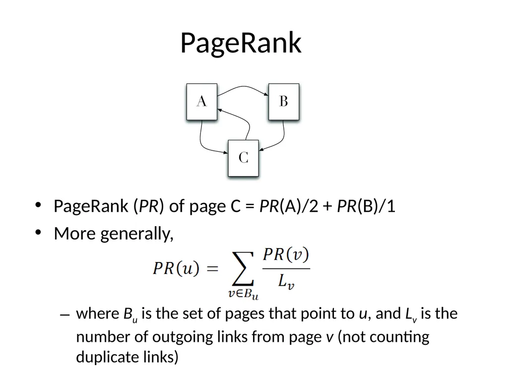
slide55. PageRank PageRank (PR) of page C = PR(A)/2 + PR(B)/1
More generally,

where Bu is the set of pages that point to u, and Lv is the number of outgoing links from page v (not counting duplicate links)<br>
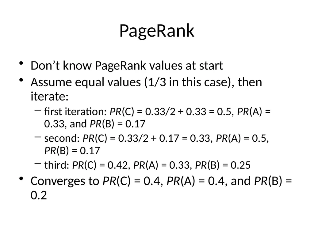
slide56. PageRank Don’t know PageRank values at start
Assume equal values (1/3 in this case), then iterate:
first iteration: PR(C) = 0.33/2 + 0.33 = 0.5, PR(A) = 0.33, and PR(B) = 0.17
second: PR(C) = 0.33/2 + 0.17 = 0.33, PR(A) = 0.5, PR(B) = 0.17
third: PR(C) = 0.42, PR(A) = 0.33, PR(B) = 0.25
Converges to PR(C) = 0.4, PR(A) = 0.4, and PR(B) = 0.2<br>
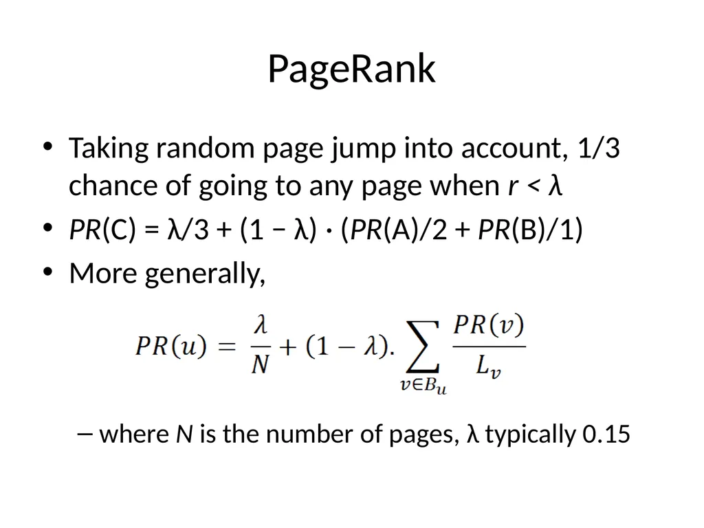
slide57. PageRank Taking random page jump into account, 1/3 chance of going to any page when r < λ
PR(C) = λ/3 + (1 − λ) · (PR(A)/2 + PR(B)/1)
More generally,

where N is the number of pages, λ typically 0.15<br>
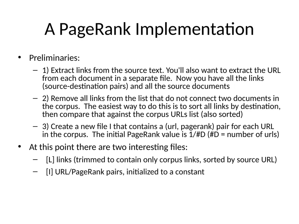
slide59. A PageRank Implementation Preliminaries:
1) Extract links from the source text. You'll also want to extract the URL from each document in a separate file. Now you have all the links (source-destination pairs) and all the source documents
2) Remove all links from the list that do not connect two documents in the corpus. The easiest way to do this is to sort all links by destination, then compare that against the corpus URLs list (also sorted)
3) Create a new file I that contains a (url, pagerank) pair for each URL in the corpus. The initial PageRank value is 1/#D (#D = number of urls)
At this point there are two interesting files:
[L] links (trimmed to contain only corpus links, sorted by source URL)
[I] URL/PageRank pairs, initialized to a constant<br>
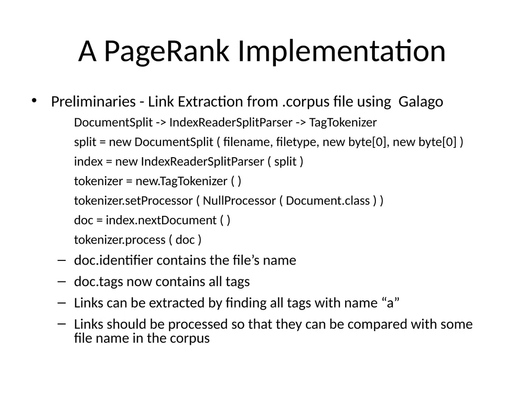
slide60. Preliminaries - Link Extraction from .corpus file using Galago
DocumentSplit -> IndexReaderSplitParser -> TagTokenizer
split = new DocumentSplit ( filename, filetype, new byte[0], new byte[0] )
index = new IndexReaderSplitParser ( split )
tokenizer = new.TagTokenizer ( )
tokenizer.setProcessor ( NullProcessor ( Document.class ) )
doc = index.nextDocument ( )
tokenizer.process ( doc )
doc.identifier contains the file’s name
doc.tags now contains all tags
Links can be extracted by finding all tags with name “a”
Links should be processed so that they can be compared with some file name in the corpus A PageRank Implementation<br>
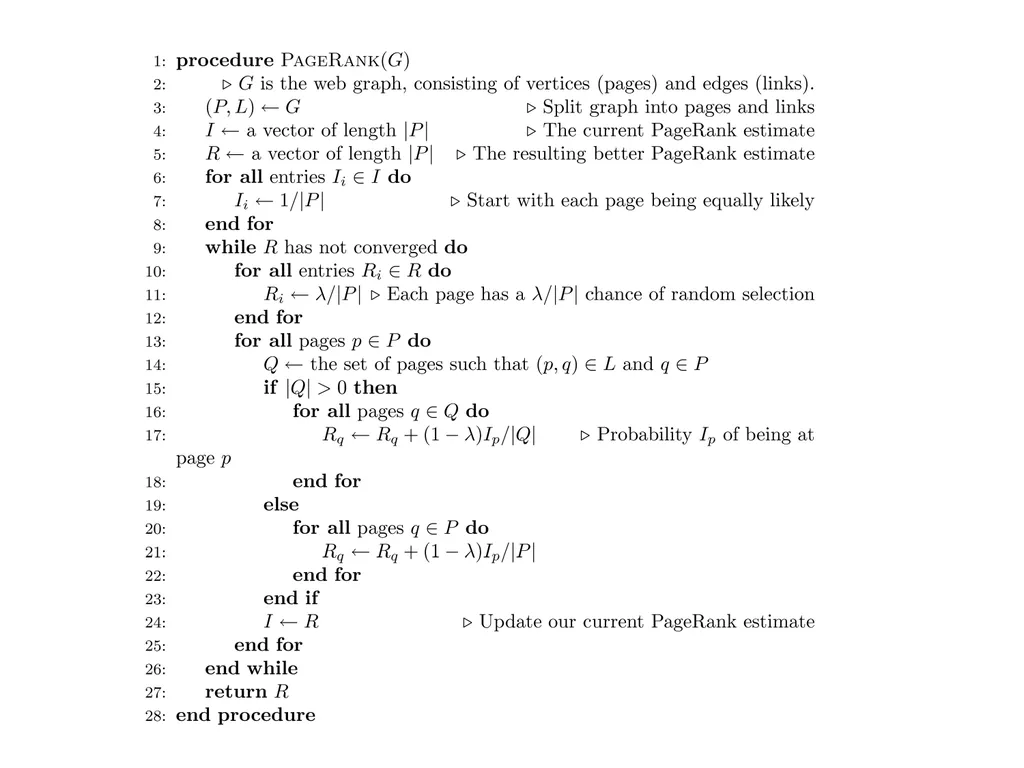
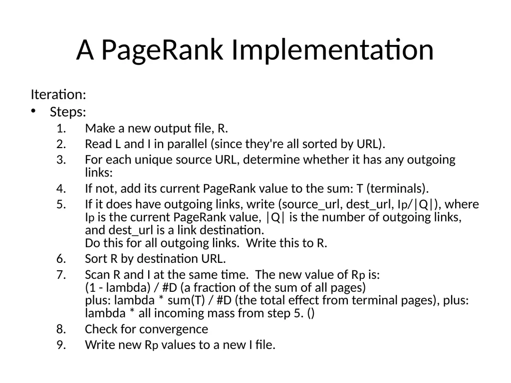
slide61. A PageRank Implementation Iteration: 
Steps:
Make a new output file, R.
Read L and I in parallel (since they're all sorted by URL).
For each unique source URL, determine whether it has any outgoing links:
If not, add its current PageRank value to the sum: T (terminals).
If it does have outgoing links, write (source_url, dest_url, Ip/|Q|), where Ip is the current PageRank value, |Q| is the number of outgoing links, and dest_url is a link destination. Do this for all outgoing links. Write this to R.
Sort R by destination URL.
Scan R and I at the same time. The new value of Rp is: (1 - lambda) / #D (a fraction of the sum of all pages)plus: lambda * sum(T) / #D (the total effect from terminal pages), plus: lambda * all incoming mass from step 5. ()
Check for convergence
Write new Rp values to a new I file.<br>
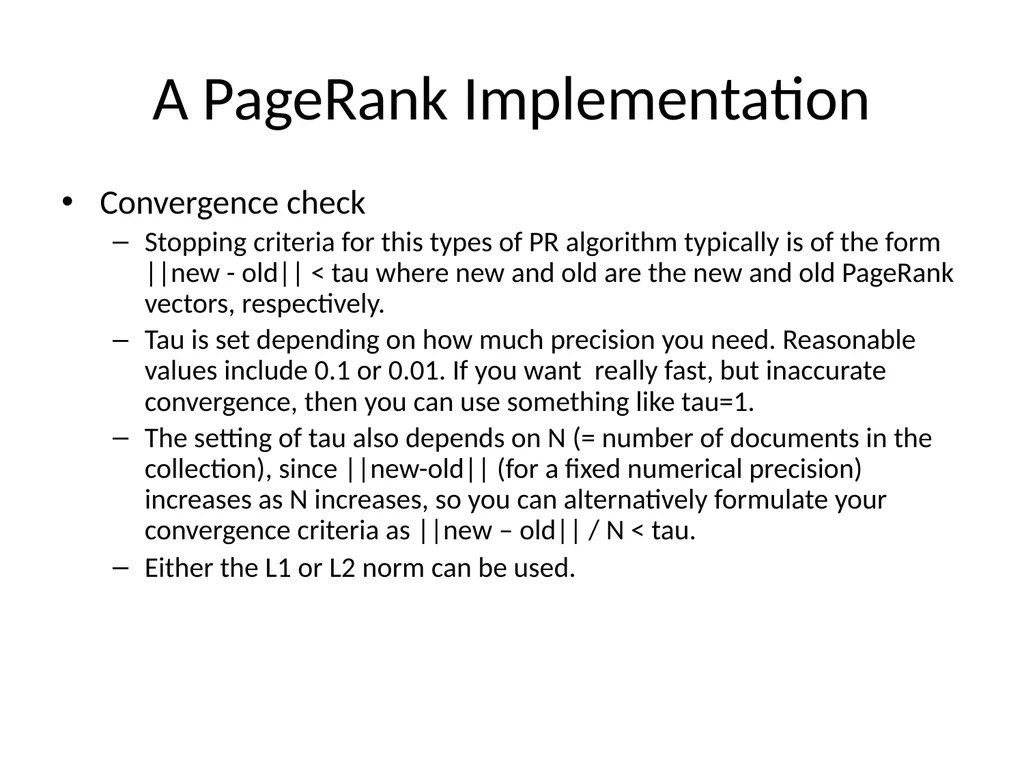
slide62. A PageRank Implementation Convergence check
Stopping criteria for this types of PR algorithm typically is of the form ||new - old|| < tau where new and old are the new and old PageRank vectors, respectively.
Tau is set depending on how much precision you need. Reasonable values include 0.1 or 0.01. If you want  really fast, but inaccurate convergence, then you can use something like tau=1.
The setting of tau also depends on N (= number of documents in the collection), since ||new-old|| (for a fixed numerical precision) increases as N increases, so you can alternatively formulate your convergence criteria as ||new – old|| / N < tau.
Either the L1 or L2 norm can be used.<br>
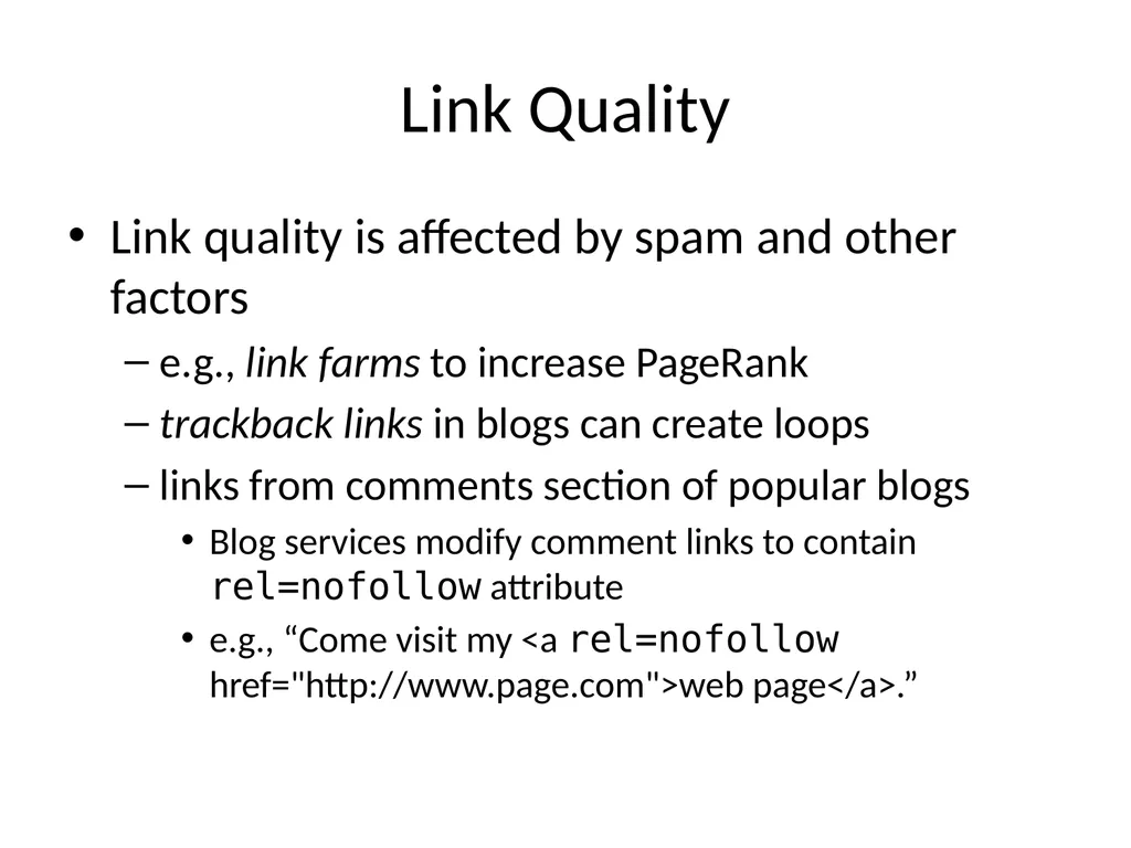
slide63. Link Quality Link quality is affected by spam and other factors
e.g., link farms to increase PageRank
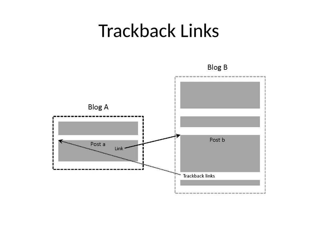
trackback links in blogs can create loops
links from comments section of popular blogs
Blog services modify comment links to contain rel=nofollow attribute
e.g., “Come visit my <a rel=nofollow href="http://www.page.com">web page</a>.”<br>
slide64. Trackback Links<br>
slide65. Information Extraction Automatically extract structure from text
annotate document using tags to identify extracted structure
Named entity recognition
identify words that refer to something of interest in a particular application
e.g., people, companies, locations, dates, product names, prices, etc.<br>
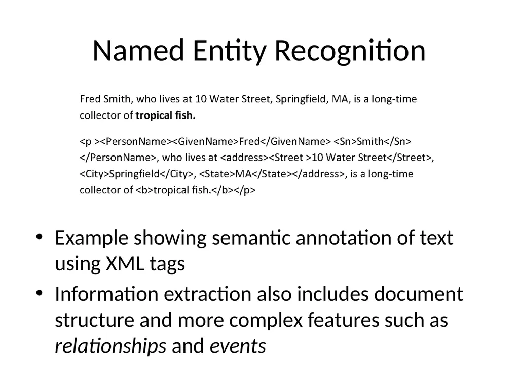
slide66. Named Entity Recognition Example showing semantic annotation of text using XML tags
Information extraction also includes document structure and more complex features such as relationships and events<br>
slide67. Named Entity Recognition Rule-based
Uses lexicons (lists of words and phrases) that categorize names
e.g., locations, peoples’ names, organizations, etc.
Rules also used to verify or find new entity names
e.g., “<number> <word> street” for addresses
“<street address>, <city>” or “in <city>” to verify city names
“<street address>, <city>, <state>” to find new cities
“<title> <name>” to find new names<br>
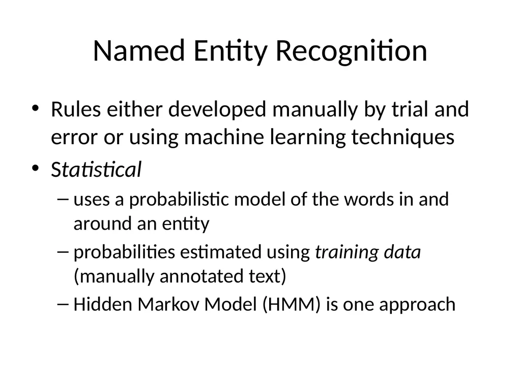
slide68. Named Entity Recognition Rules either developed manually by trial and error or using machine learning techniques
Statistical
uses a probabilistic model of the words in and around an entity
probabilities estimated using training data (manually annotated text)
Hidden Markov Model (HMM) is one approach<br>
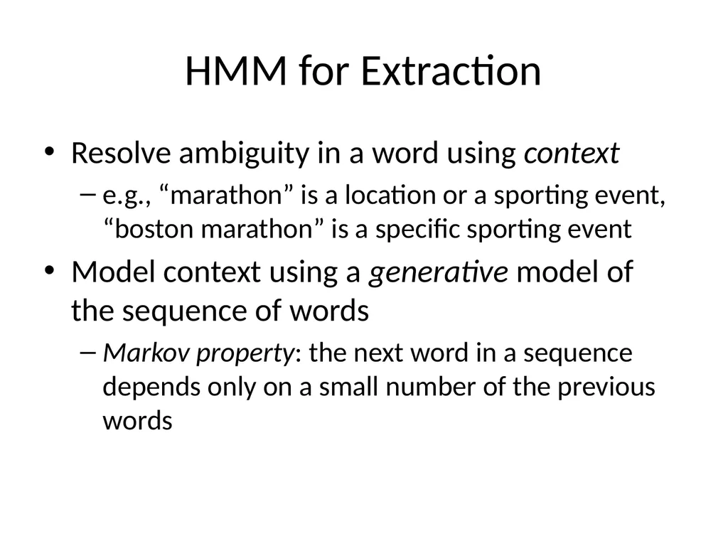
slide69. HMM for Extraction Resolve ambiguity in a word using context
e.g., “marathon” is a location or a sporting event, “boston marathon” is a specific sporting event
Model context using a generative model of the sequence of words
Markov property: the next word in a sequence depends only on a small number of the previous words<br>
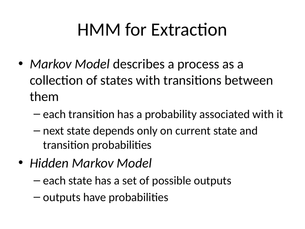
slide70. HMM for Extraction Markov Model describes a process as a collection of states with transitions between them
each transition has a probability associated with it
next state depends only on current state and transition probabilities
Hidden Markov Model
each state has a set of possible outputs
outputs have probabilities<br>
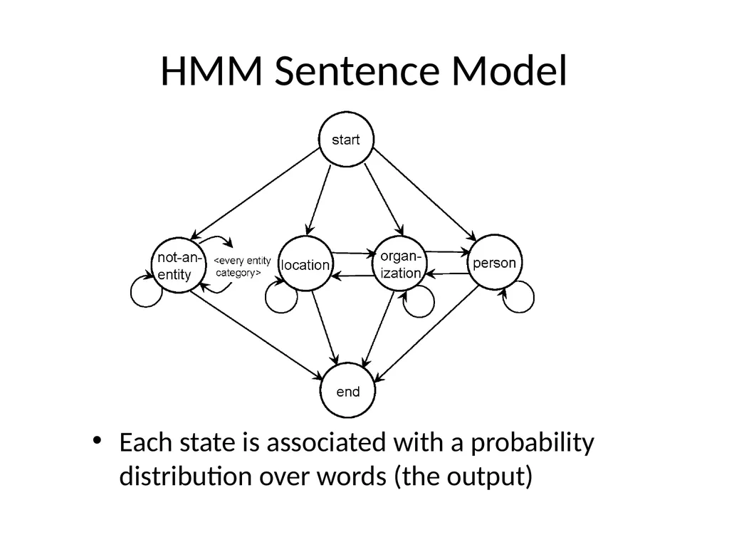
slide71. HMM Sentence Model Each state is associated with a probability distribution over words (the output)<br>
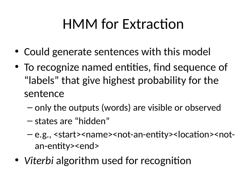
slide72. HMM for Extraction Could generate sentences with this model
To recognize named entities, find sequence of “labels” that give highest probability for the sentence
only the outputs (words) are visible or observed
states are “hidden”
e.g., <start><name><not-an-entity><location><not-an-entity><end>
Viterbi algorithm used for recognition<br>
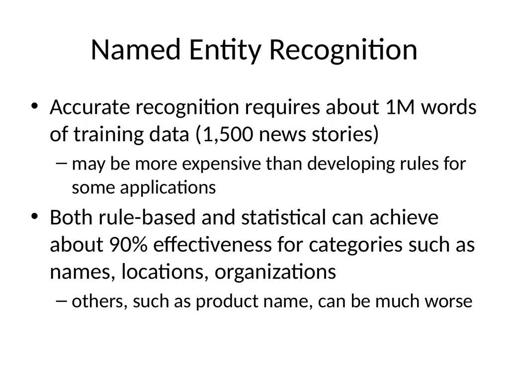
slide73. Named Entity Recognition Accurate recognition requires about 1M words of training data (1,500 news stories)
may be more expensive than developing rules for some applications
Both rule-based and statistical can achieve about 90% effectiveness for categories such as names, locations, organizations
others, such as product name, can be much worse<br>
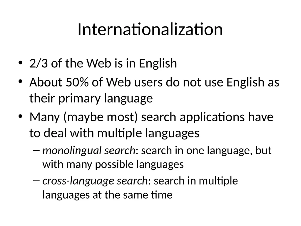
slide74. Internationalization 2/3 of the Web is in English
About 50% of Web users do not use English as their primary language
Many (maybe most) search applications have to deal with multiple languages
monolingual search: search in one language, but with many possible languages
cross-language search: search in multiple languages at the same time<br>
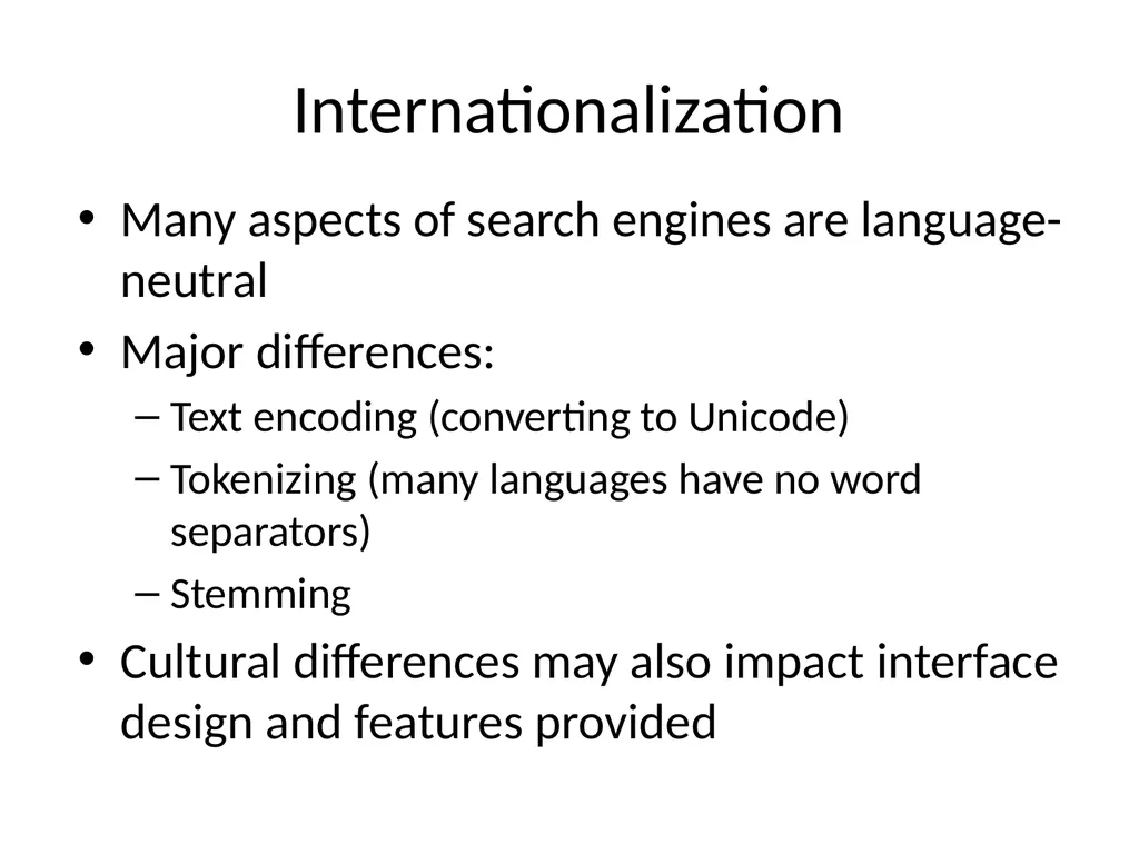
slide75. Internationalization Many aspects of search engines are language-neutral
Major differences:
Text encoding (converting to Unicode)
Tokenizing (many languages have no word separators)
Stemming
Cultural differences may also impact interface design and features provided<br>
slide76. Chinese “Tokenizing”<br>