Shelly Cashman: Microsoft Excel 2019 Module 2:

lois-ondreau

Published 2026-09-28 · 42 slides · 0 views

↓ Download

Shelly Cashman: Microsoft Excel 2019 Module 2:

Shelly Cashman: Microsoft Excel 2019 Module 2: - slide 1 of 42

Shelly Cashman: Microsoft Excel 2019 Module 2: - slide 2 of 42

Shelly Cashman: Microsoft Excel 2019 Module 2: - slide 3 of 42

Shelly Cashman: Microsoft Excel 2019 Module 2: - slide 4 of 42

Shelly Cashman: Microsoft Excel 2019 Module 2: - slide 5 of 42

Shelly Cashman: Microsoft Excel 2019 Module 2: - slide 6 of 42

Shelly Cashman: Microsoft Excel 2019 Module 2: - slide 7 of 42

Shelly Cashman: Microsoft Excel 2019 Module 2: - slide 8 of 42

Shelly Cashman: Microsoft Excel 2019 Module 2: - slide 9 of 42

Shelly Cashman: Microsoft Excel 2019 Module 2: - slide 10 of 42

Shelly Cashman: Microsoft Excel 2019 Module 2: - slide 11 of 42

Shelly Cashman: Microsoft Excel 2019 Module 2: - slide 12 of 42

Shelly Cashman: Microsoft Excel 2019 Module 2: - slide 13 of 42

Shelly Cashman: Microsoft Excel 2019 Module 2: - slide 17 of 42

Shelly Cashman: Microsoft Excel 2019 Module 2: - slide 18 of 42

Shelly Cashman: Microsoft Excel 2019 Module 2: - slide 19 of 42

Shelly Cashman: Microsoft Excel 2019 Module 2: - slide 20 of 42

Shelly Cashman: Microsoft Excel 2019 Module 2: - slide 21 of 42

Shelly Cashman: Microsoft Excel 2019 Module 2: - slide 22 of 42

Shelly Cashman: Microsoft Excel 2019 Module 2: - slide 23 of 42

Shelly Cashman: Microsoft Excel 2019 Module 2: - slide 24 of 42

Shelly Cashman: Microsoft Excel 2019 Module 2: - slide 25 of 42

Shelly Cashman: Microsoft Excel 2019 Module 2: - slide 26 of 42

Shelly Cashman: Microsoft Excel 2019 Module 2: - slide 27 of 42

Shelly Cashman: Microsoft Excel 2019 Module 2: - slide 28 of 42

Shelly Cashman: Microsoft Excel 2019 Module 2: - slide 29 of 42

Shelly Cashman: Microsoft Excel 2019 Module 2: - slide 30 of 42

Shelly Cashman: Microsoft Excel 2019 Module 2: - slide 31 of 42

Shelly Cashman: Microsoft Excel 2019 Module 2: - slide 32 of 42

Shelly Cashman: Microsoft Excel 2019 Module 2: - slide 33 of 42

Shelly Cashman: Microsoft Excel 2019 Module 2: - slide 34 of 42

Shelly Cashman: Microsoft Excel 2019 Module 2: - slide 35 of 42

Shelly Cashman: Microsoft Excel 2019 Module 2: - slide 36 of 42

Shelly Cashman: Microsoft Excel 2019 Module 2: - slide 37 of 42

Shelly Cashman: Microsoft Excel 2019 Module 2: - slide 38 of 42

Shelly Cashman: Microsoft Excel 2019 Module 2: - slide 39 of 42

Shelly Cashman: Microsoft Excel 2019 Module 2: - slide 40 of 42

Shelly Cashman: Microsoft Excel 2019 Module 2: - slide 41 of 42

Shelly Cashman: Microsoft Excel 2019 Module 2: - slide 42 of 42

Description

Shelly Cashman: Microsoft Excel 2019 Module 2: Formulas, Functions, and Formatting 2020 Cengage Learning. All Rights Reserved. May not be copied, scanned, or duplicated, in whole or in part, except for use as permitted in a license

Download this presentation From Below

"Shelly Cashman: Microsoft Excel 2019 Module 2:" is the property of its rightful owner. Permission is granted to download and print the materials on this website for personal, non-commercial use only, and to display it on your personal computer provided you do not modify the materials and that you retain all copyright notices contained in the materials. By downloading content from our website, you accept the terms of this agreement.

Presentation Transcript

Shelly Cashman: Microsoft Excel 2019 Module 2: Formulas, Functions, and Formatting © 2020 Cengage Learning. All Rights Reserved. May not be copied, scanned, or duplicated, in whole or in part, except for use as permitted in a license distributed with a certain product or service or otherwise on a password-protected website for classroom use.

Objectives (1 of 2) Use Flash Fill
Enter formulas using the keyboard
Enter formulas using Point mode
Apply the MAX, MIN, and AVERAGE functions
Verify a formula using Range Finder
Apply a theme to a workbook
Apply a date format to a cell or range

Objectives (2 of 2) Add conditional formatting to cells
Change column width and row height
Check the spelling on a worksheet
Change margins and headers in Page Layout view
Preview and print versions and sections of a worksheet

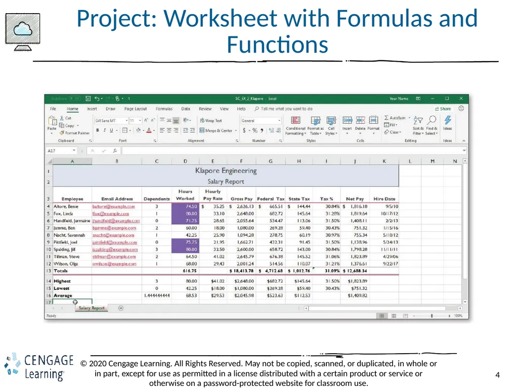
Project: Worksheet with Formulas and Functions

Entering the Titles and Numbers into the Worksheet (1 of 2) To Enter the Worksheet Title and Subtitle
Run Excel and create a blank workbook
Select cell A1 and type the desired text, then press the DOWN ARROW key to enter the worksheet title
Select cell A2 and type the desired then press the DOWN ARROW key to enter the worksheet subtitle
To Enter the Column Titles
Select cell A3 and type the desired text, then press the RIGHT ARROW key to enter the column heading
Continue until all the columns you desire have headings

Entering the Titles and Numbers into the Worksheet (2 of 2) To Enter the Salary Data
Use the data in Table 2-1 to enter salary data in a worksheet
Select cell A4, type desired name, and then press the RIGHT ARROW key two times to enter the employee name and make cell C4 the active cell
Type a number in cell C4 and then press the RIGHT ARROW key
Type a number of hours worked in cell D4 and then press the RIGHT ARROW key
Type an hourly rate in cell E4
Click cell K4 and type a date

Flash Fill (1 of 2) To Use Flash Fill
Click a cell
Type desired text and then press the DOWN ARROW to select the next cell
Type desired text again following the same pattern (for example an email address)
Click Data on the ribbon to select the Data tab
Click Flash Fill to enter similarly formatted text

Flash Fill (2 of 2) To Enter the Row Titles
Select a cell in the A column
Type desired text and then press the DOWN ARROW key to enter a row header.
Continue until all Rows have a header
To Change the Sheet Tab Name and Color
Double-click the Sheet1 tab and enter the desired text as the sheet tab name and then press the ENTER key
Right-click the sheet tab to display the shortcut menu
Point to Tab Color on the shortcut menu to display the Tab Color gallery. Click desired color
Save the workbook

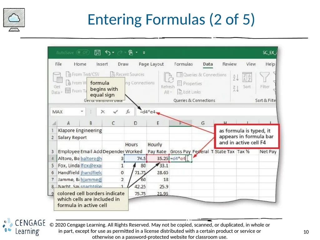
Entering Formulas (1 of 5) To Enter a Formula Using the Keyboard
With the cell to contain the formula selected, type the formula in the cell to display the formula in the formula bar and in the current cell and to display colored borders around the cells referenced in the formula
Press TAB to complete the arithmetic operation indicated by the formula, to display the result in the worksheet, and to select the cell to the right

Entering Formulas (2 of 5)

Entering Formulas (3 of 5) Order of Operations
From left to right
First negation (−)
Then percentages (%)
Then all exponentiations (^)
Then all multiplications (*) and divisions (/)
Finally all additions (+) and subtractions (−)

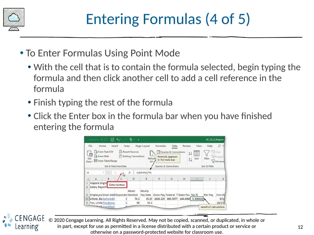
Entering Formulas (4 of 5) To Enter Formulas Using Point Mode
With the cell that is to contain the formula selected, begin typing the formula and then click another cell to add a cell reference in the formula
Finish typing the rest of the formula
Click the Enter box in the formula bar when you have finished entering the formula

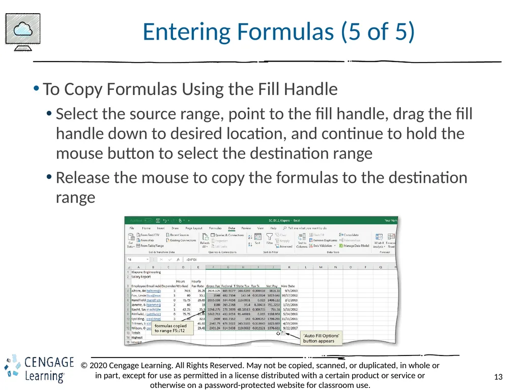
Entering Formulas (5 of 5) To Copy Formulas Using the Fill Handle
Select the source range, point to the fill handle, drag the fill handle down to desired location, and continue to hold the mouse button to select the destination range
Release the mouse to copy the formulas to the destination range

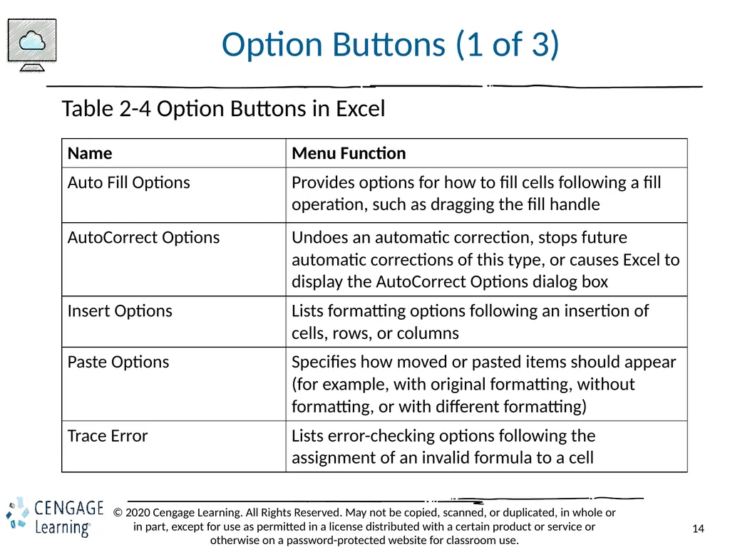
Option Buttons (1 of 3) Table 2-4 Option Buttons in Excel

Option Buttons (2 of 3) To Determine Totals Using the AutoSum Button
Display the Home tab
Select the desired cell to contain the sum, click the AutoSum button to sum the contents of the range and click ENTER to display the total in the selected cell
Select the range to contain the sums. Click the AutoSum button to display totals in the selected range
Select the cell to contain the sum, click the AutoSum button to sum the contents of the range and click ENTER

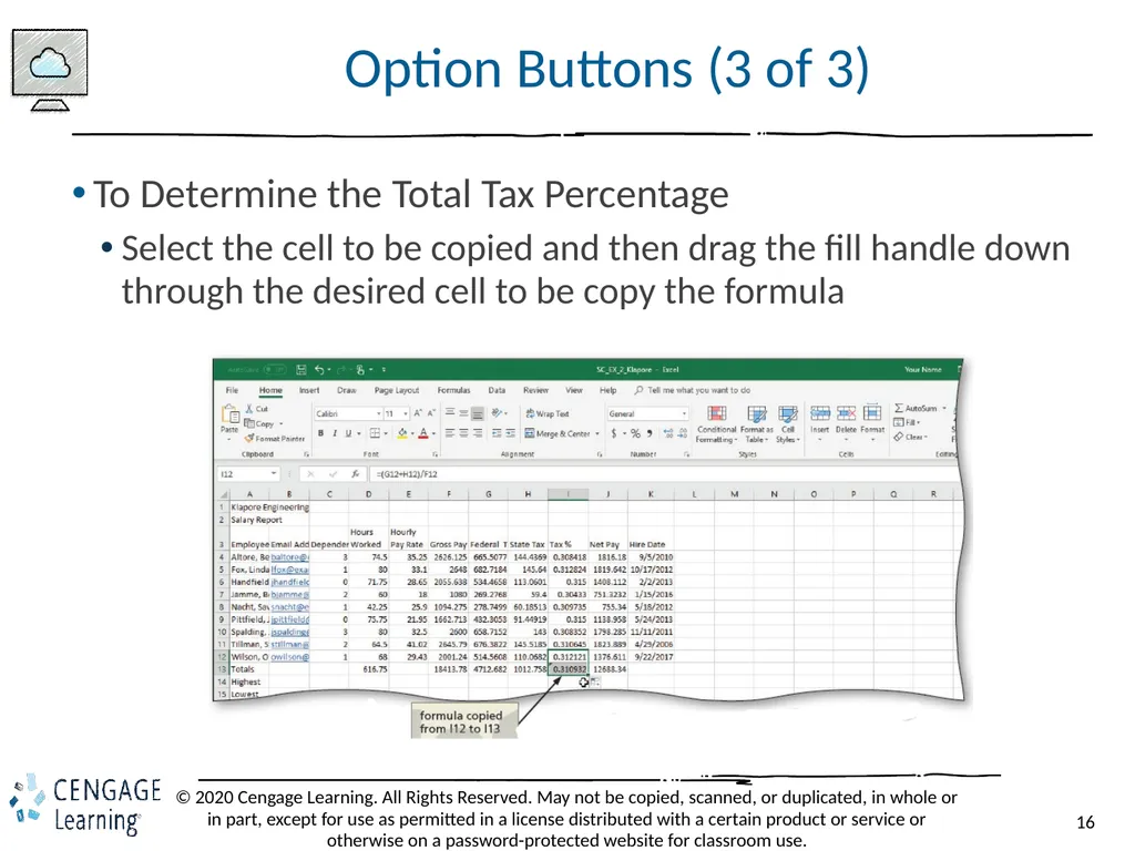
Option Buttons (3 of 3) To Determine the Total Tax Percentage
Select the cell to be copied and then drag the fill handle down through the desired cell to be copy the formula

Using the AVERAGE, MAX, MIN, and other Statistical Functions (1 of 6) To Determine the Highest Number in a Range of Numbers Using the Insert Function Dialog box
Select the cell to contain the maximum number
Click the Insert Function box in the formula bar to display the Insert Function dialog box
If necessary, scroll to and then click MAX in the Select a function list
Click the OK button to display the Function Arguments dialog box and type the cell range in the Number1 box to enter the first argument of the function
Click the OK button to display the highest value in the chosen range in the selected cell

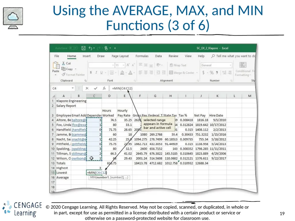
Using the AVERAGE, MAX, and MIN Functions (2 of 6) To Determine the Lowest Number in a Range of Numbers Using the Sum Menu
Select cell that is to contain the minimum value and then click the AutoSum arrow in the HOME tab
Click Min to display the MIN function in the formula bar and in the active cell
Drag through the range of values of which you want to determine the lowest number
Click the Enter box to determine the lowest value in the range and display the result in the formula bar and in the selected cell

Using the AVERAGE, MAX, and MIN Functions (3 of 6)

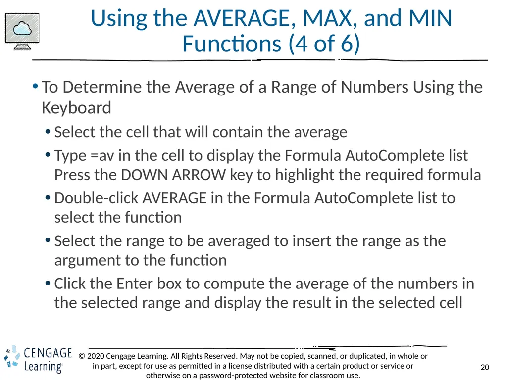
Using the AVERAGE, MAX, and MIN Functions (4 of 6) To Determine the Average of a Range of Numbers Using the Keyboard
Select the cell that will contain the average
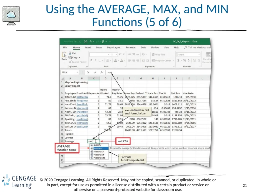
Type =av in the cell to display the Formula AutoComplete list Press the DOWN ARROW key to highlight the required formula
Double-click AVERAGE in the Formula AutoComplete list to select the function
Select the range to be averaged to insert the range as the argument to the function
Click the Enter box to compute the average of the numbers in the selected range and display the result in the selected cell

Using the AVERAGE, MAX, and MIN Functions (5 of 6)

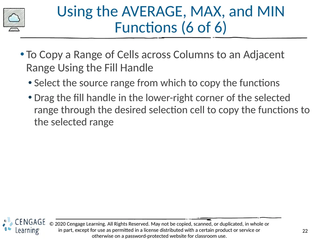
Using the AVERAGE, MAX, and MIN Functions (6 of 6) To Copy a Range of Cells across Columns to an Adjacent Range Using the Fill Handle
Select the source range from which to copy the functions
Drag the fill handle in the lower-right corner of the selected range through the desired selection cell to copy the functions to the selected range

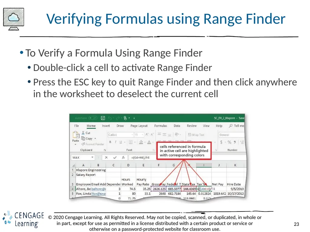
Verifying Formulas using Range Finder To Verify a Formula Using Range Finder
Double-click a cell to activate Range Finder
Press the ESC key to quit Range Finder and then click anywhere in the worksheet to deselect the current cell

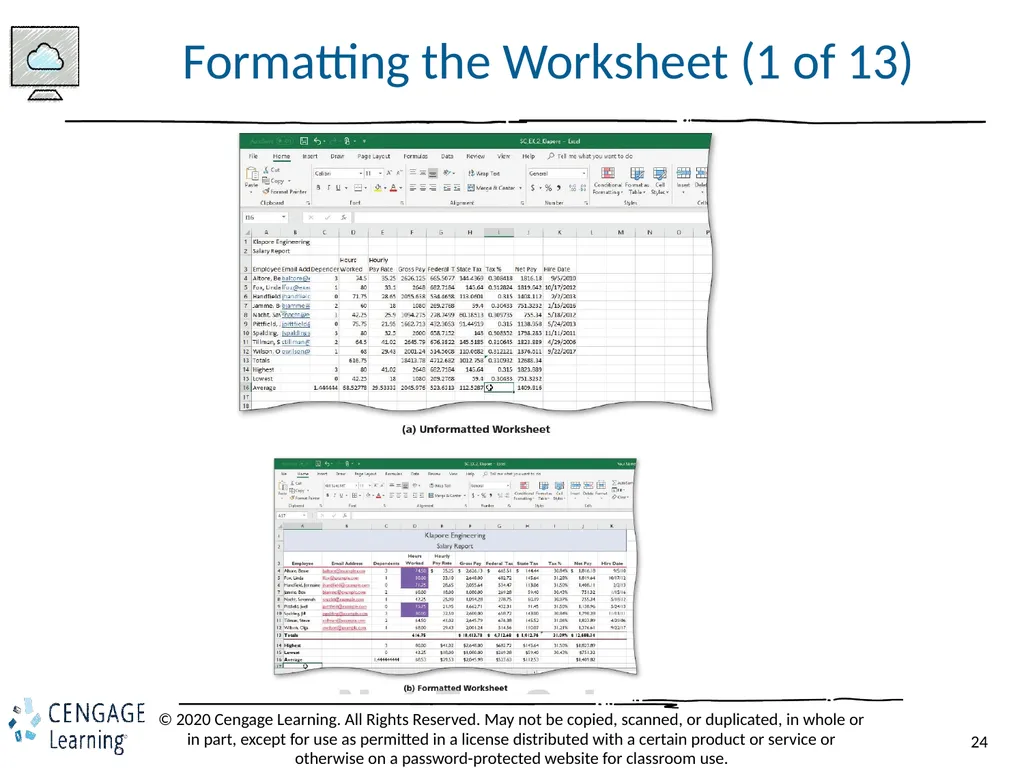
Formatting the Worksheet (1 of 13)

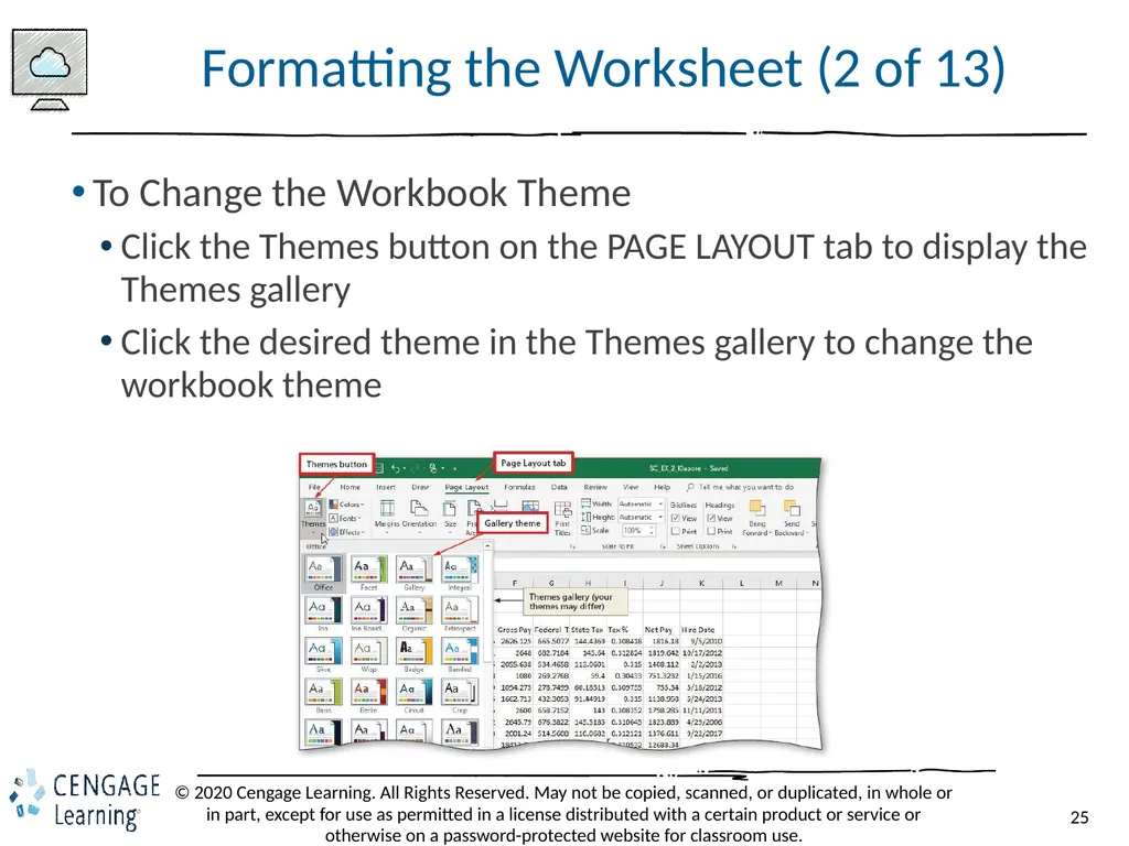
Formatting the Worksheet (2 of 13) To Change the Workbook Theme
Click the Themes button on the PAGE LAYOUT tab to display the Themes gallery
Click the desired theme in the Themes gallery to change the workbook theme

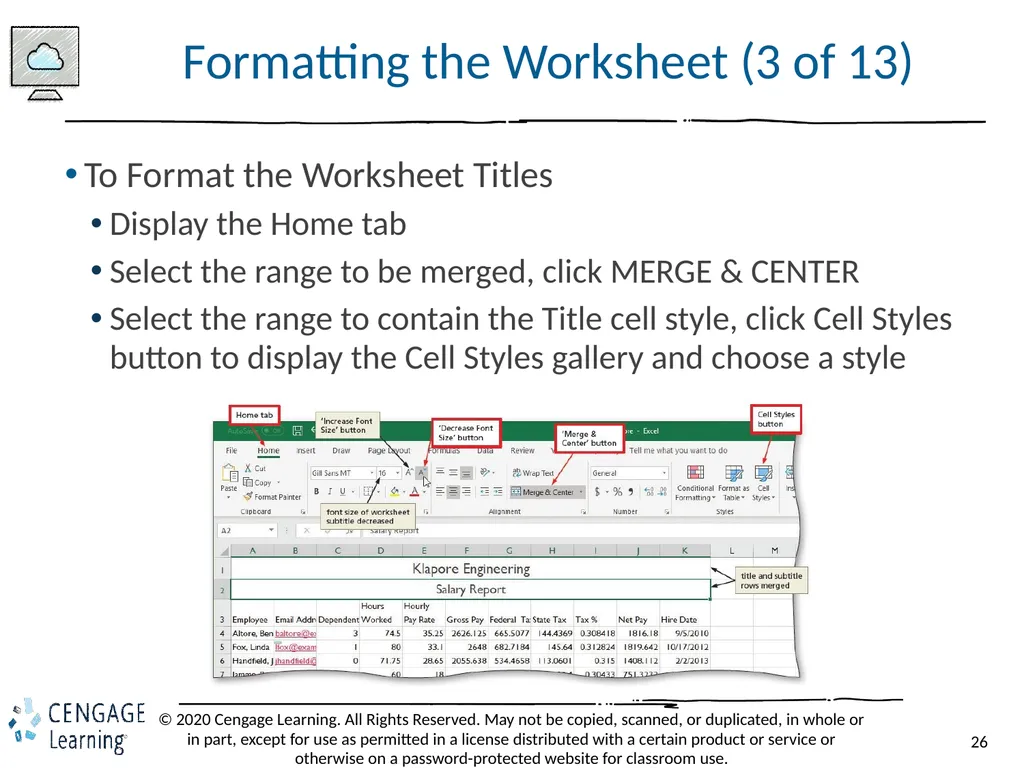
Formatting the Worksheet (3 of 13) To Format the Worksheet Titles
Display the Home tab
Select the range to be merged, click MERGE & CENTER
Select the range to contain the Title cell style, click Cell Styles button to display the Cell Styles gallery and choose a style

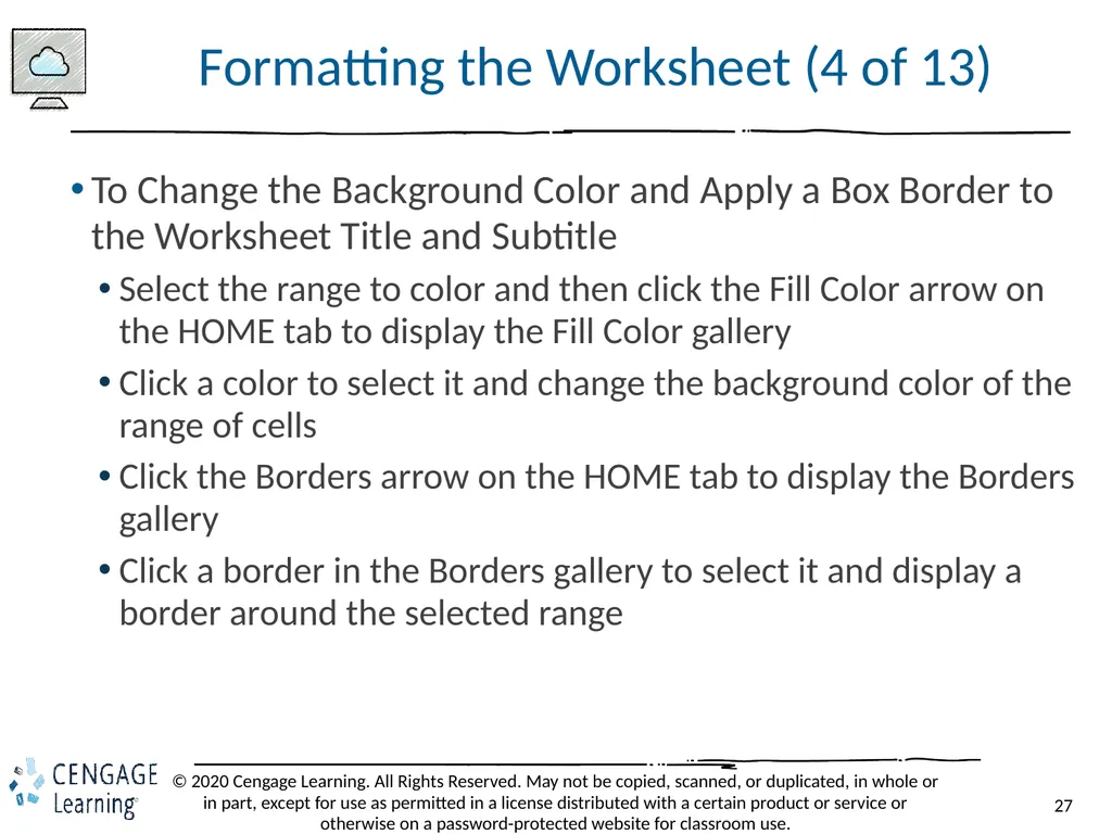
Formatting the Worksheet (4 of 13) To Change the Background Color and Apply a Box Border to the Worksheet Title and Subtitle
Select the range to color and then click the Fill Color arrow on the HOME tab to display the Fill Color gallery
Click a color to select it and change the background color of the range of cells
Click the Borders arrow on the HOME tab to display the Borders gallery
Click a border in the Borders gallery to select it and display a border around the selected range

Formatting the Worksheet (5 of 13) To Apply a Cell Style to the Column Headings and Format the Total Rows
Select the range to be formatted
Use the Cell Styles gallery to apply the cell style
Click the Center button to center the column headings
Apply the Total cell style to the range
Bold the range

Formatting the Worksheet (6 of 13) To Format Dates and Center Data in Cells
Select the range to contain the new date format
On the HOME tab in the Number group, click the Dialog Box Launcher to display the Format Cells dialog box
If necessary, click the NUMBER tab and click Date in the Category list, and then click a date type to choose the format for the selected range
Click the OK button to format the dates in the current column using the selected date format style
Select the range to be centered and then click the Center button on the HOME tab to center the data in the selected range

Formatting the Worksheet (7 of 13) To Apply an Accounting Number Format and Comma Style Format Using the Ribbon
Select the range to contain the accounting number format
While holding down the CTRL key, select the nonadjacent ranges and cells
Click the “Accounting Number Format” button on the HOME tab to apply the accounting number format to the selected nonadjacent ranges
Click the Comma Style button on the HOME tab to assign the Comma style format to the selected range

Formatting the Worksheet (8 of 13) To Apply a Currency Style Format with a Floating Dollar Sign Using the Format Cells Dialog Box
Select the range to format and then on the HOME tab in the Number group, click the Dialog Box Launcher to display the Format Cells dialog box
If necessary, click the NUMBER tab to display the Number sheet
Click Currency in the Category list to select the necessary number format category and then tap or click a style in the Negative numbers list to select the desired currency format
Click the OK button to assign the currency style format to the selected ranges

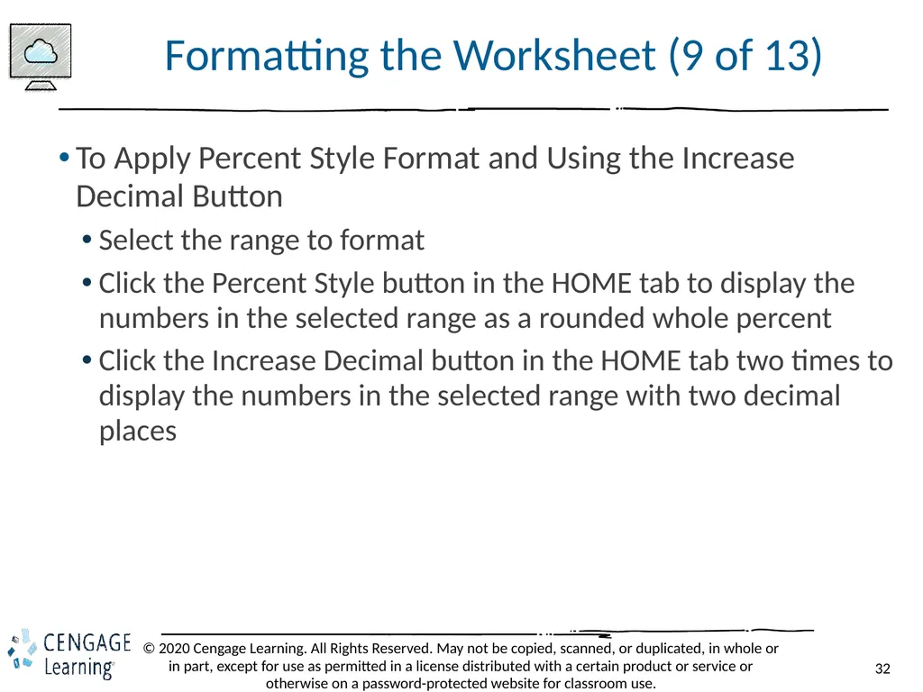
Formatting the Worksheet (9 of 13) To Apply Percent Style Format and Using the Increase Decimal Button
Select the range to format
Click the Percent Style button in the HOME tab to display the numbers in the selected range as a rounded whole percent
Click the Increase Decimal button in the HOME tab two times to display the numbers in the selected range with two decimal places

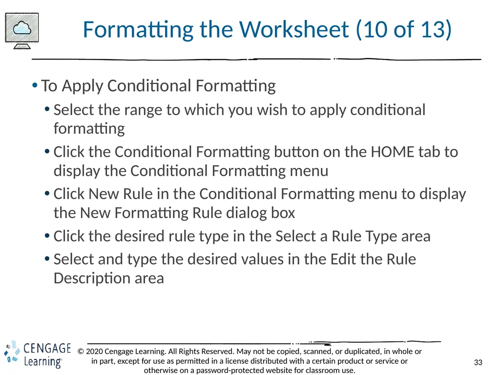
Formatting the Worksheet (10 of 13) To Apply Conditional Formatting
Select the range to which you wish to apply conditional formatting
Click the Conditional Formatting button on the HOME tab to display the Conditional Formatting menu
Click New Rule in the Conditional Formatting menu to display the New Formatting Rule dialog box
Click the desired rule type in the Select a Rule Type area
Select and type the desired values in the Edit the Rule Description area

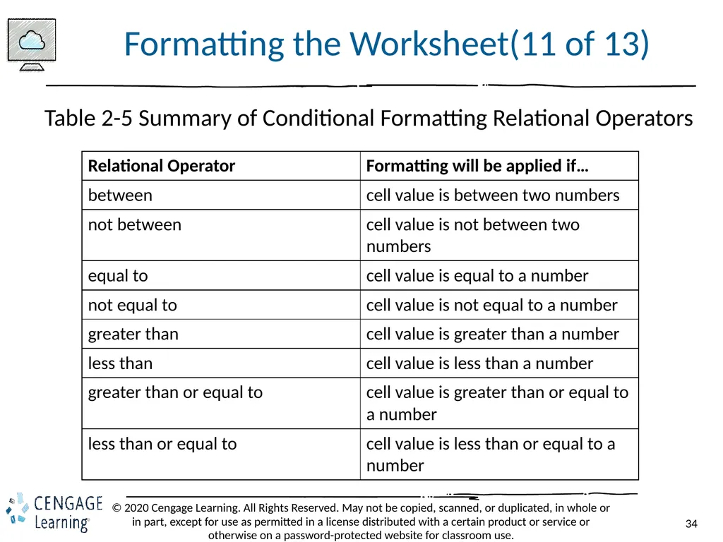
Formatting the Worksheet(11 of 13) Table 2-5 Summary of Conditional Formatting Relational Operators

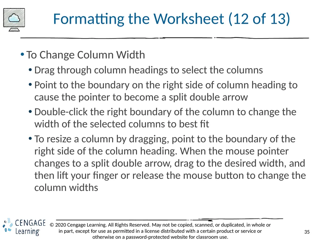
Formatting the Worksheet (12 of 13) To Change Column Width
Drag through column headings to select the columns
Point to the boundary on the right side of column heading to cause the pointer to become a split double arrow
Double-click the right boundary of the column to change the width of the selected columns to best fit
To resize a column by dragging, point to the boundary of the right side of the column heading. When the mouse pointer changes to a split double arrow, drag to the desired width, and then lift your finger or release the mouse button to change the column widths

Formatting the Worksheet (13 of 13) To Change the Row Height
Point to the boundary below the row heading to resize
Drag the boundary to the desired row height and then release the mouse button
Lift your finger or release the mouse button to change the row height

Checking Spelling To Check Spelling on the Worksheet
Click cell A1 so that the spell checker begins at the beginning of the worksheet
Click the Spelling button on the REVIEW tab to run the spell checker and display the misspelled words in the Spelling dialog box
Apply the desired action to each misspelled word
When the spell checker is finished, click the Close button

Printing the Worksheet (1 of 3) To Change the Worksheet’s Margins, Header, and Orientation in Page Layout View
Click the Page Layout button on the status bar to view the worksheet in Page Layout view
Click the Adjust Margins button on the PAGE LAYOUT tab to display the Margins gallery
Click the desired margin style to change the worksheet margins to the selected style
Click above cell A1 in the center area of the Header area
Type the desired worksheet header, and then press the ENTER key
Click the “Change Page Orientation” button on the PAGE LAYOUT tab to display the Change Page Orientation gallery
Click the desired orientation in the Orientation gallery to change the worksheet’s orientation

Printing the Worksheet (2 of 3) To Print a Worksheet
Click FILE on the ribbon to open Backstage view
Click the Print to display the Print screen
If necessary, click Printer Status button to display a list of available printer and click the desired printer
Click the No Scaling button and then select “Fit Sheet on One Page”
Click Print

Printing the Worksheet (3 of 3) To Print a Section of the Worksheet
Select the range to print
Click FILE on the ribbon to open Backstage view
Click the Print to display the Print screen
Click “Print Active Sheets” in the Settings area on the PRINT screen to display a list of printing options
Click Print Selection to print the selected range
Click the Print button in the Print screen to print the selected range of the worksheet
Click the Normal button on the status bar to return to Normal view

Displaying and Printing the Formulas Version of the Worksheet (1 of 2) To Display the Formulas in the Worksheet and Fit the Printout on One Page
Press CTRL+ACCENT MARK (`) to display the worksheet with formulas
Click the Page Setup Dialog Box Launcher on the PAGE LAYOUT tab to display the Page Setup dialog box
If necessary, click the desired Orientation in the Page sheet to select it
If necessary, click Fit to in the Scaling area to select it
Click the Print button to open the Print screen in Backstage view. Select the Print Selection button in the Settings area of the Print gallery and then click Print Active Sheets
Click the Print button to print the worksheet
After viewing and printing the formulas version, press CTRL+ACCENT MARK (`) to display the values version

Displaying and Printing the Formulas Version of the Worksheet (2 of 2) To Change the Print Scaling Option Back to 100%
Click the Page Setup Dialog Box Launcher on the PAGE LAYOUT tab to display the Page Setup dialog box
Click the Adjust to option button in the Scaling area to select the Adjust to setting
If necessary, type 100 in the Adjust to box to adjust the print scaling to 100%
Click OK
Display the Home tab
Save the workbook, sign out and exit Excel

Shelly Cashman: Microsoft Excel 2019 Module 2:

Related Topics

Share

Embed code

Download this presentation From Below

Presentation Transcript