
Shelly Cashman: Microsoft Excel 2019 Module 3:
AS
Published · 50 slides · 0 views
1 / 1
Description
Shelly Cashman: Microsoft Excel 2019 Module 3: Working with Large Worksheets, Charting, and What-If Analysis 2020 Cengage Learning. All Rights Reserved. May not be copied, scanned, or duplicated, in whole or in part, except for use as
Related Topics
Share
Embed code
Download this presentation From Below
"Shelly Cashman: Microsoft Excel 2019 Module 3:" is the property of its rightful owner. Permission is granted to download and print the materials on this website for personal, non-commercial use only, and to display it on your personal computer provided you do not modify the materials and that you retain all copyright notices contained in the materials. By downloading content from our website, you accept the terms of this agreement.
Presentation Transcript
01
Shelly Cashman: Microsoft Excel 2019 Module 3: Working with Large Worksheets, Charting, and What-If Analysis © 2020 Cengage Learning. All Rights Reserved. May not be copied, scanned, or duplicated, in whole or in part, except for use as permitted in a license distributed with a certain product or service or otherwise on a password-protected website for classroom use.<br>
02
Objectives (1 of 2) Rotate text in a cell
Create a series of month names
Copy, paste, insert, and delete cells
Format numbers using format symbols
Enter and format the system date
Use absolute and mixed cell references in a formula
Use the IF function to perform a logical test
Create and format sparkline charts
Change sparkline chart types and styles
Use the Format Painter button to format cells<br>
Create a series of month names
Copy, paste, insert, and delete cells
Format numbers using format symbols
Enter and format the system date
Use absolute and mixed cell references in a formula
Use the IF function to perform a logical test
Create and format sparkline charts
Change sparkline chart types and styles
Use the Format Painter button to format cells<br>
03
Objectives (2 of 2) Create a clustered column chart on a separate chart sheet
Use chart filters to display a subset of data in a chart
Change the chart style and type
Reorder sheet tabs
Change the worksheet view
Freeze and unfreeze rows and columns
Answer what-if questions
Goal seek to answer what-if questions
Use Smart Lookup
Understand accessibility features<br>
Use chart filters to display a subset of data in a chart
Change the chart style and type
Reorder sheet tabs
Change the worksheet view
Freeze and unfreeze rows and columns
Answer what-if questions
Goal seek to answer what-if questions
Use Smart Lookup
Understand accessibility features<br>
04
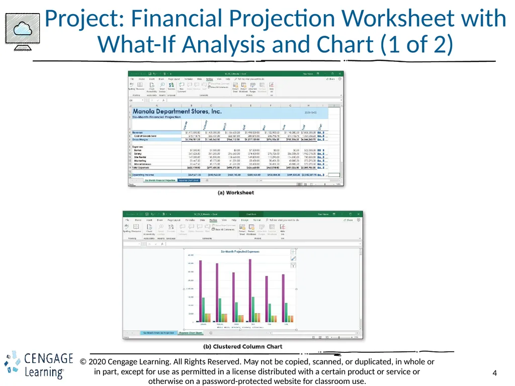
Project: Financial Projection Worksheet with What-If Analysis and Chart (1 of 2)<br>
05
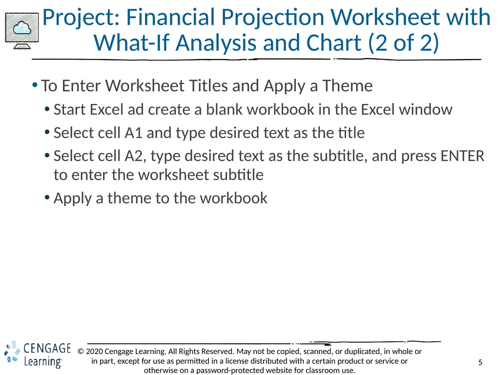
Project: Financial Projection Worksheet with What-If Analysis and Chart (2 of 2) To Enter Worksheet Titles and Apply a Theme
Start Excel ad create a blank workbook in the Excel window
Select cell A1 and type desired text as the title
Select cell A2, type desired text as the subtitle, and press ENTER to enter the worksheet subtitle
Apply a theme to the workbook<br>
Start Excel ad create a blank workbook in the Excel window
Select cell A1 and type desired text as the title
Select cell A2, type desired text as the subtitle, and press ENTER to enter the worksheet subtitle
Apply a theme to the workbook<br>
06
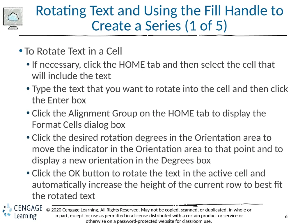
Rotating Text and Using the Fill Handle to Create a Series (1 of 5) To Rotate Text in a Cell
If necessary, click the HOME tab and then select the cell that will include the text
Type the text that you want to rotate into the cell and then click the Enter box
Click the Alignment Group on the HOME tab to display the Format Cells dialog box
Click the desired rotation degrees in the Orientation area to move the indicator in the Orientation area to that point and to display a new orientation in the Degrees box
Click the OK button to rotate the text in the active cell and automatically increase the height of the current row to best fit the rotated text<br>
If necessary, click the HOME tab and then select the cell that will include the text
Type the text that you want to rotate into the cell and then click the Enter box
Click the Alignment Group on the HOME tab to display the Format Cells dialog box
Click the desired rotation degrees in the Orientation area to move the indicator in the Orientation area to that point and to display a new orientation in the Degrees box
Click the OK button to rotate the text in the active cell and automatically increase the height of the current row to best fit the rotated text<br>
07
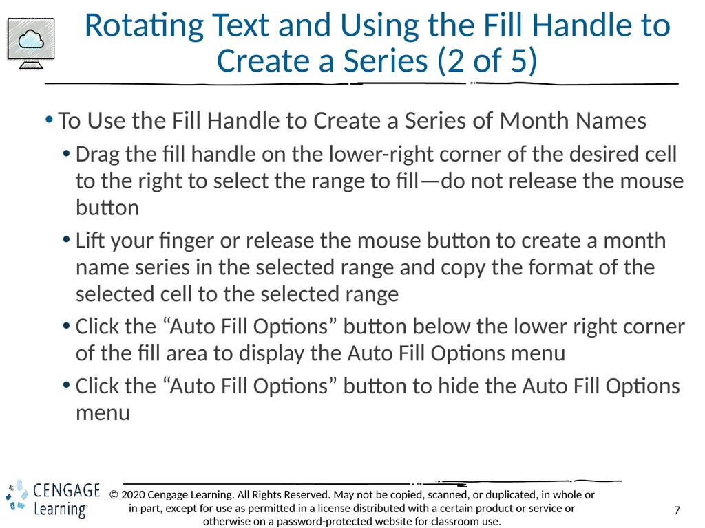
Rotating Text and Using the Fill Handle to Create a Series (2 of 5) To Use the Fill Handle to Create a Series of Month Names
Drag the fill handle on the lower-right corner of the desired cell to the right to select the range to fill—do not release the mouse button
Lift your finger or release the mouse button to create a month name series in the selected range and copy the format of the selected cell to the selected range
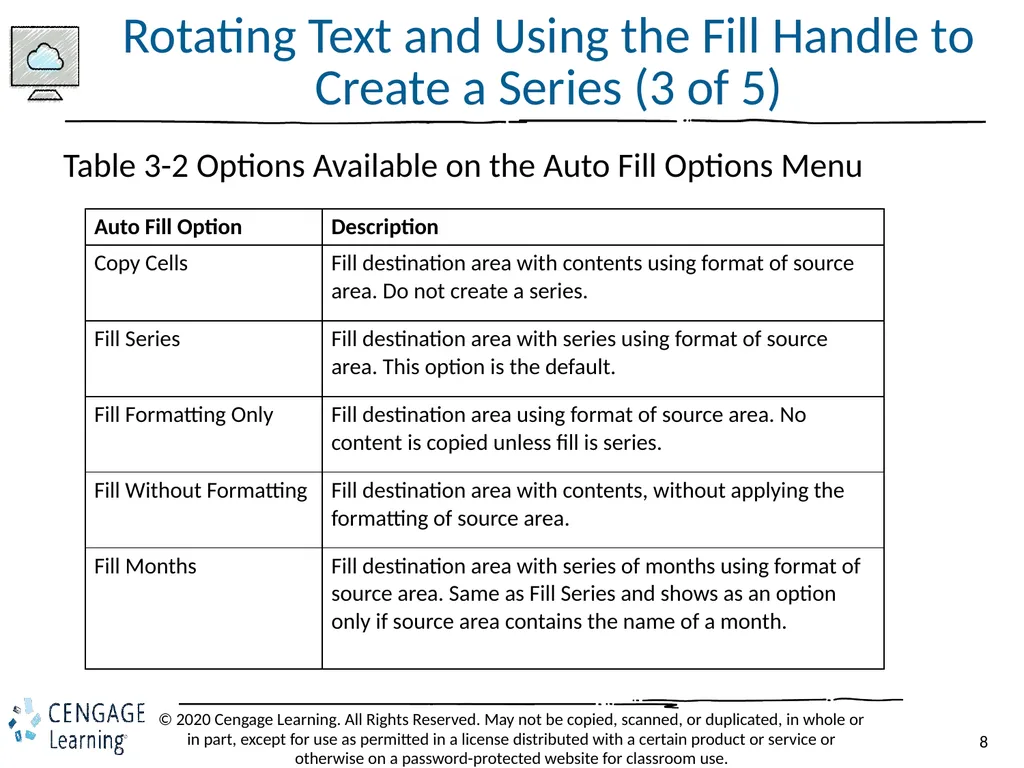
Click the “Auto Fill Options” button below the lower right corner of the fill area to display the Auto Fill Options menu
Click the “Auto Fill Options” button to hide the Auto Fill Options menu<br>
Drag the fill handle on the lower-right corner of the desired cell to the right to select the range to fill—do not release the mouse button
Lift your finger or release the mouse button to create a month name series in the selected range and copy the format of the selected cell to the selected range
Click the “Auto Fill Options” button below the lower right corner of the fill area to display the Auto Fill Options menu
Click the “Auto Fill Options” button to hide the Auto Fill Options menu<br>
08
Rotating Text and Using the Fill Handle to Create a Series (3 of 5) Table 3-2 Options Available on the Auto Fill Options Menu<br>
09
Rotating Text and Using the Fill Handle to Create a Series (4 of 5) To Increase Column Widths
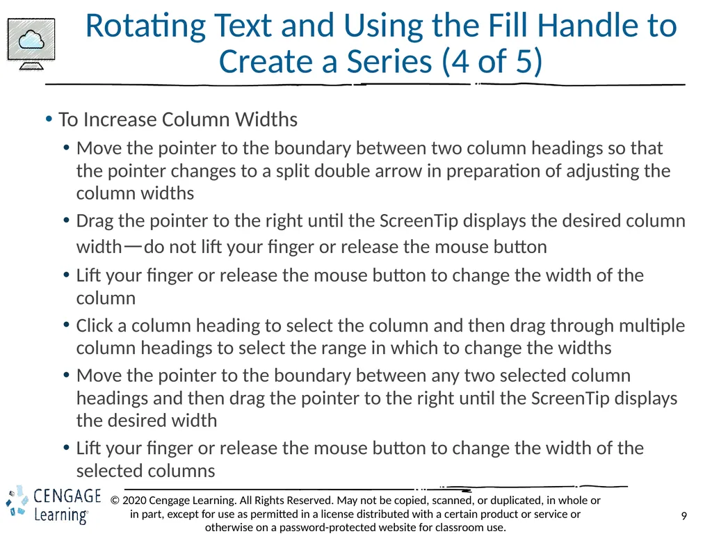
Move the pointer to the boundary between two column headings so that the pointer changes to a split double arrow in preparation of adjusting the column widths
Drag the pointer to the right until the ScreenTip displays the desired column width—do not lift your finger or release the mouse button
Lift your finger or release the mouse button to change the width of the column
Click a column heading to select the column and then drag through multiple column headings to select the range in which to change the widths
Move the pointer to the boundary between any two selected column headings and then drag the pointer to the right until the ScreenTip displays the desired width
Lift your finger or release the mouse button to change the width of the selected columns<br>
Move the pointer to the boundary between two column headings so that the pointer changes to a split double arrow in preparation of adjusting the column widths
Drag the pointer to the right until the ScreenTip displays the desired column width—do not lift your finger or release the mouse button
Lift your finger or release the mouse button to change the width of the column
Click a column heading to select the column and then drag through multiple column headings to select the range in which to change the widths
Move the pointer to the boundary between any two selected column headings and then drag the pointer to the right until the ScreenTip displays the desired width
Lift your finger or release the mouse button to change the width of the selected columns<br>
10
Rotating Text and Using the Fill Handle to Create a Series (5 of 5) To Enter and Indent Row Titles
Select the cell to which you want to apply the indent
Click the Increase Indent button on the HOME tab to increase the indentation of the text in the selected cell
Select a range of cells and then click the Increase Indent button on the HOME tab to increase the indentation of the text in the selected range<br>
Select the cell to which you want to apply the indent
Click the Increase Indent button on the HOME tab to increase the indentation of the text in the selected cell
Select a range of cells and then click the Increase Indent button on the HOME tab to increase the indentation of the text in the selected range<br>
11
Copying a Range of Cells to a Nonadjacent Destination Area To Copy a Range of Cells to a Nonadjacent Destination Area
Select the cell or range of cells to copy, and then click the Copy button on the HOME tab to copy the values and formats of the selected range to the Office Clipboard
Click the first cell in the destination area
Click the Paste button on the HOME tab to copy the values and formats of the last item placed on the Office Clipboard to the destination area<br>
Select the cell or range of cells to copy, and then click the Copy button on the HOME tab to copy the values and formats of the selected range to the Office Clipboard
Click the first cell in the destination area
Click the Paste button on the HOME tab to copy the values and formats of the last item placed on the Office Clipboard to the destination area<br>
12
Inserting and Deleting Cells in a Worksheet (1 of 4) To Insert a Row
Right-click the row heading below where you want to insert a row to display the shortcut menu and the mini toolbar
Click Insert on the shortcut menu to insert a new row in the worksheet by shifting the selected row and all rows below it down one row<br>
Right-click the row heading below where you want to insert a row to display the shortcut menu and the mini toolbar
Click Insert on the shortcut menu to insert a new row in the worksheet by shifting the selected row and all rows below it down one row<br>
13
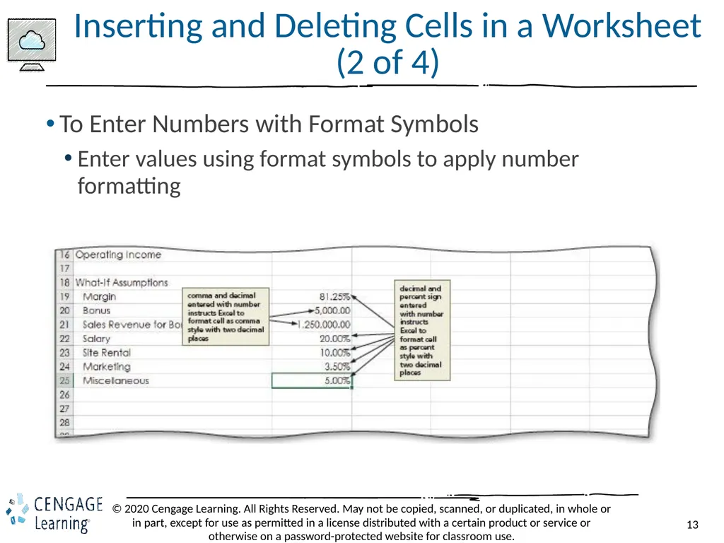
Inserting and Deleting Cells in a Worksheet (2 of 4) To Enter Numbers with Format Symbols
Enter values using format symbols to apply number formatting<br>
Enter values using format symbols to apply number formatting<br>
14
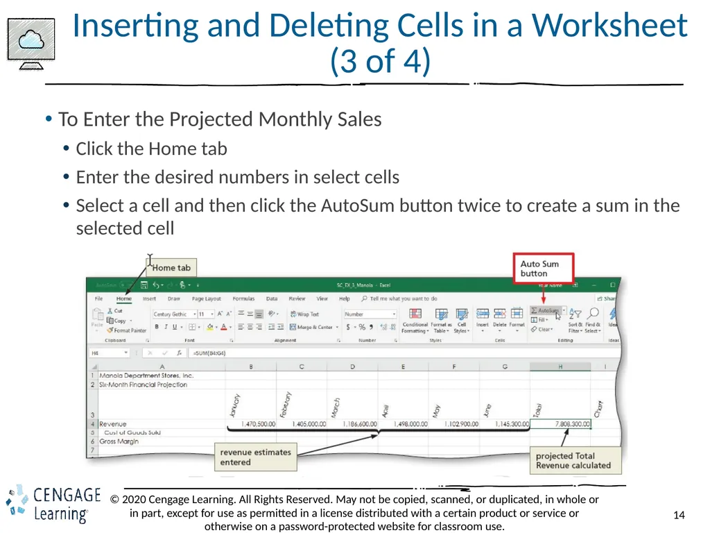
Inserting and Deleting Cells in a Worksheet (3 of 4) To Enter the Projected Monthly Sales
Click the Home tab
Enter the desired numbers in select cells
Select a cell and then click the AutoSum button twice to create a sum in the selected cell<br>
Click the Home tab
Enter the desired numbers in select cells
Select a cell and then click the AutoSum button twice to create a sum in the selected cell<br>
15
Inserting and Deleting Cells in a Worksheet (4 of 4) To Enter and Format the System Date
Select the cell in which you want to insert the date, and then click the Insert Function box in the formula bar to display the Insert Function dialog box
Click the “Or select a category” arrow and then select “Date & Time” in the list to populate the “Select a function” list with date and time functions
Scroll down in the “Select a function list” and then click NOW to select the function
Click the OK button to close the Insert Function dialog box
Click the OK button to display the system date and time in the selected cell<br>
Select the cell in which you want to insert the date, and then click the Insert Function box in the formula bar to display the Insert Function dialog box
Click the “Or select a category” arrow and then select “Date & Time” in the list to populate the “Select a function” list with date and time functions
Scroll down in the “Select a function list” and then click NOW to select the function
Click the OK button to close the Insert Function dialog box
Click the OK button to display the system date and time in the selected cell<br>
16
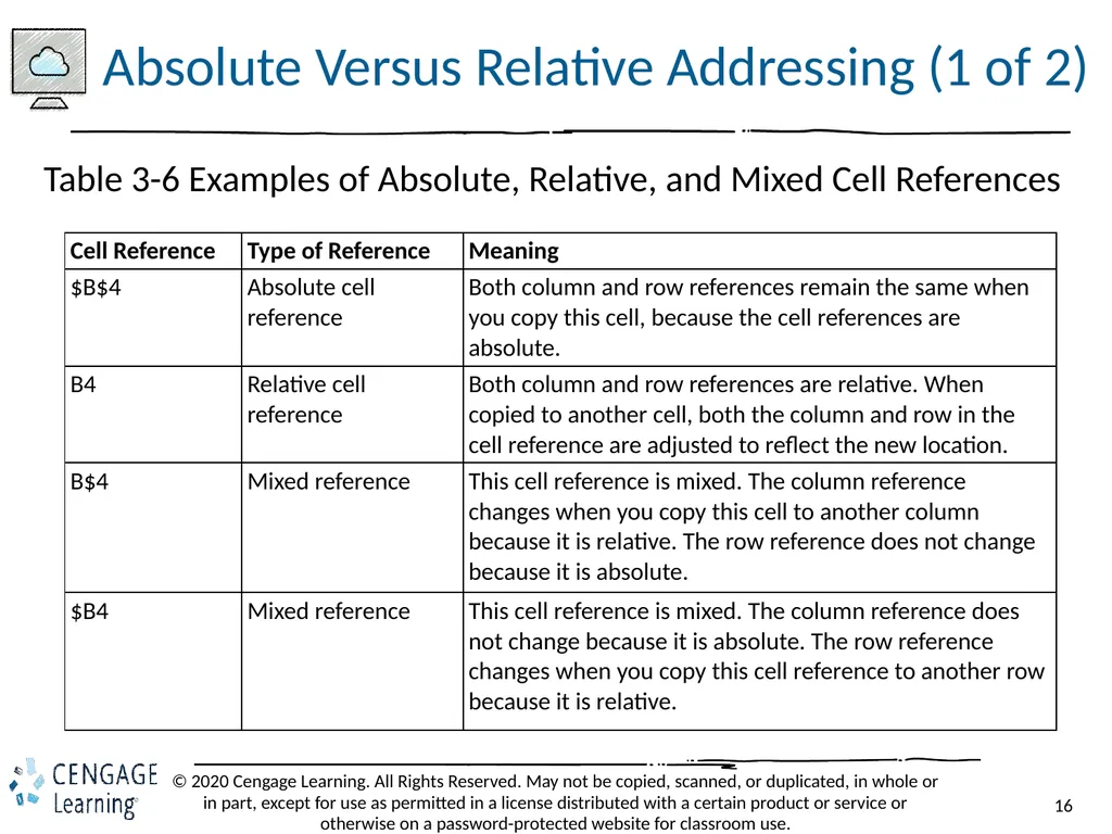
Absolute Versus Relative Addressing (1 of 2) Table 3-6 Examples of Absolute, Relative, and Mixed Cell References<br>
17
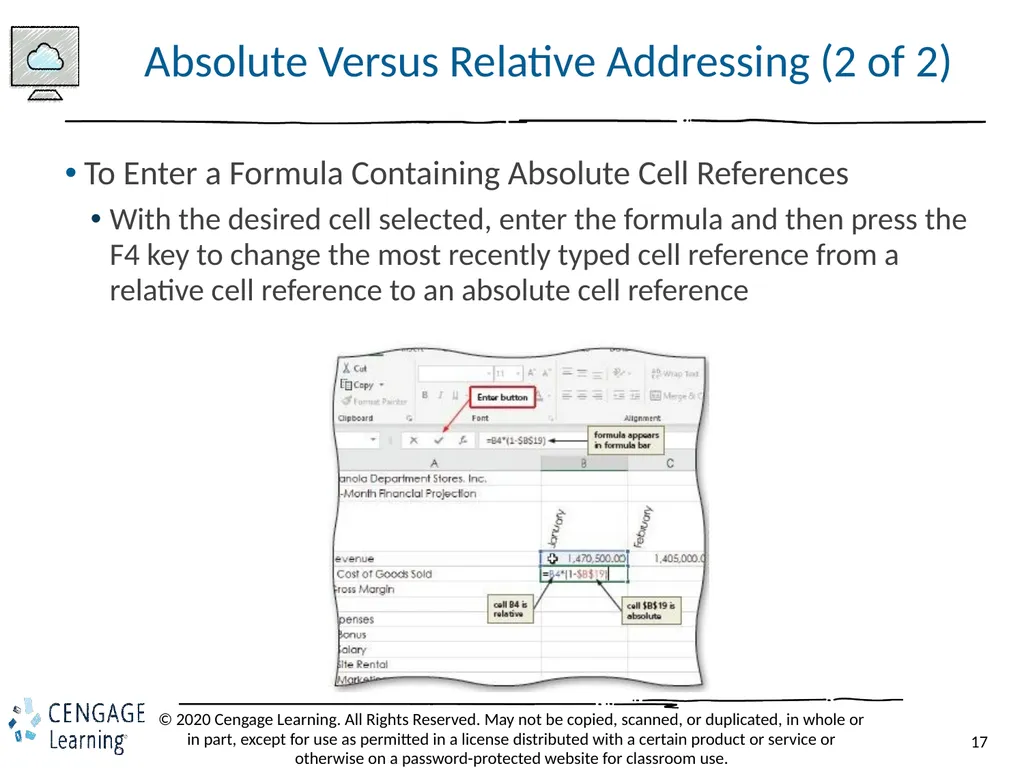
Absolute Versus Relative Addressing (2 of 2) To Enter a Formula Containing Absolute Cell References
With the desired cell selected, enter the formula and then press the F4 key to change the most recently typed cell reference from a relative cell reference to an absolute cell reference<br>
With the desired cell selected, enter the formula and then press the F4 key to change the most recently typed cell reference from a relative cell reference to an absolute cell reference<br>
18
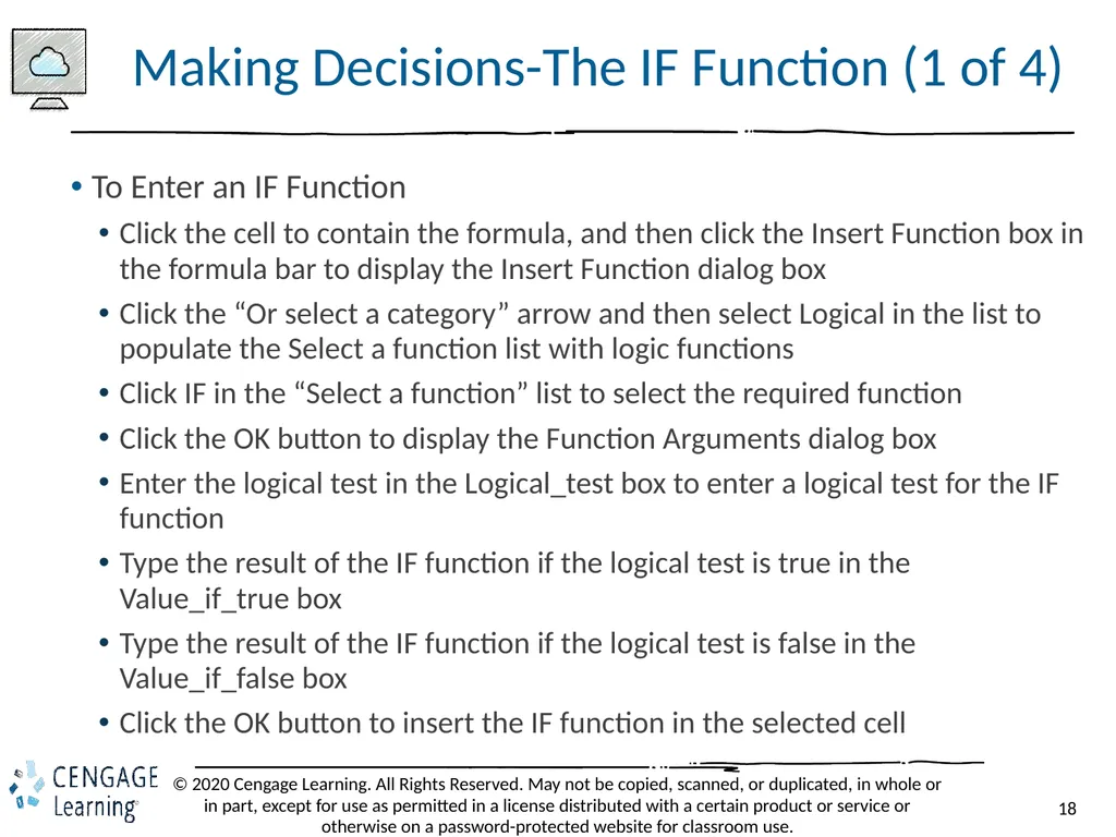
Making Decisions-The IF Function (1 of 4) To Enter an IF Function
Click the cell to contain the formula, and then click the Insert Function box in the formula bar to display the Insert Function dialog box
Click the “Or select a category” arrow and then select Logical in the list to populate the Select a function list with logic functions
Click IF in the “Select a function” list to select the required function
Click the OK button to display the Function Arguments dialog box
Enter the logical test in the Logical_test box to enter a logical test for the IF function
Type the result of the IF function if the logical test is true in the Value_if_true box
Type the result of the IF function if the logical test is false in the Value_if_false box
Click the OK button to insert the IF function in the selected cell<br>
Click the cell to contain the formula, and then click the Insert Function box in the formula bar to display the Insert Function dialog box
Click the “Or select a category” arrow and then select Logical in the list to populate the Select a function list with logic functions
Click IF in the “Select a function” list to select the required function
Click the OK button to display the Function Arguments dialog box
Enter the logical test in the Logical_test box to enter a logical test for the IF function
Type the result of the IF function if the logical test is true in the Value_if_true box
Type the result of the IF function if the logical test is false in the Value_if_false box
Click the OK button to insert the IF function in the selected cell<br>
19
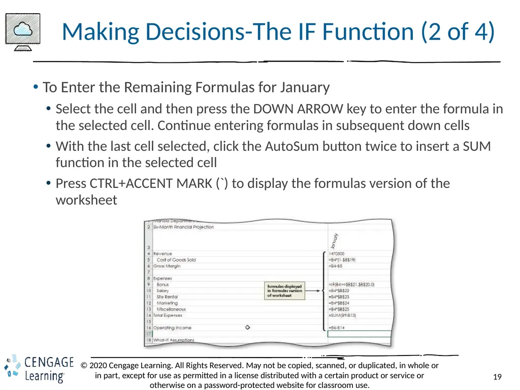
Making Decisions-The IF Function (2 of 4) To Enter the Remaining Formulas for January
Select the cell and then press the DOWN ARROW key to enter the formula in the selected cell. Continue entering formulas in subsequent down cells
With the last cell selected, click the AutoSum button twice to insert a SUM function in the selected cell
Press CTRL+ACCENT MARK (`) to display the formulas version of the worksheet<br>
Select the cell and then press the DOWN ARROW key to enter the formula in the selected cell. Continue entering formulas in subsequent down cells
With the last cell selected, click the AutoSum button twice to insert a SUM function in the selected cell
Press CTRL+ACCENT MARK (`) to display the formulas version of the worksheet<br>
20
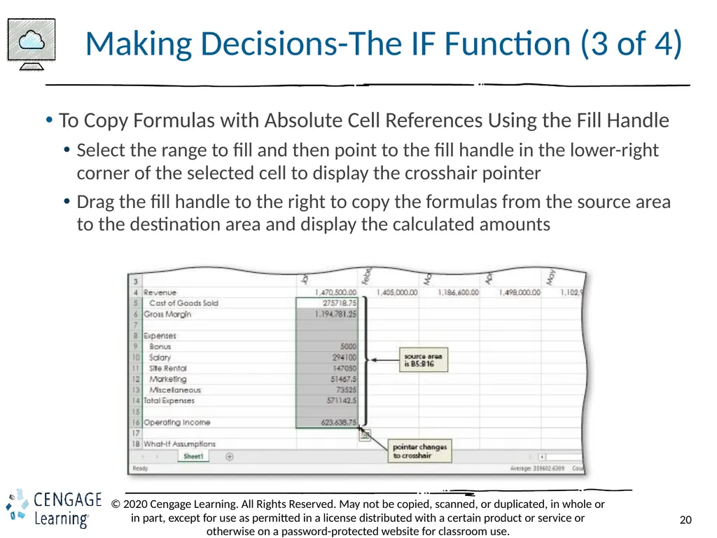
Making Decisions-The IF Function (3 of 4) To Copy Formulas with Absolute Cell References Using the Fill Handle
Select the range to fill and then point to the fill handle in the lower-right corner of the selected cell to display the crosshair pointer
Drag the fill handle to the right to copy the formulas from the source area to the destination area and display the calculated amounts<br>
Select the range to fill and then point to the fill handle in the lower-right corner of the selected cell to display the crosshair pointer
Drag the fill handle to the right to copy the formulas from the source area to the destination area and display the calculated amounts<br>
21
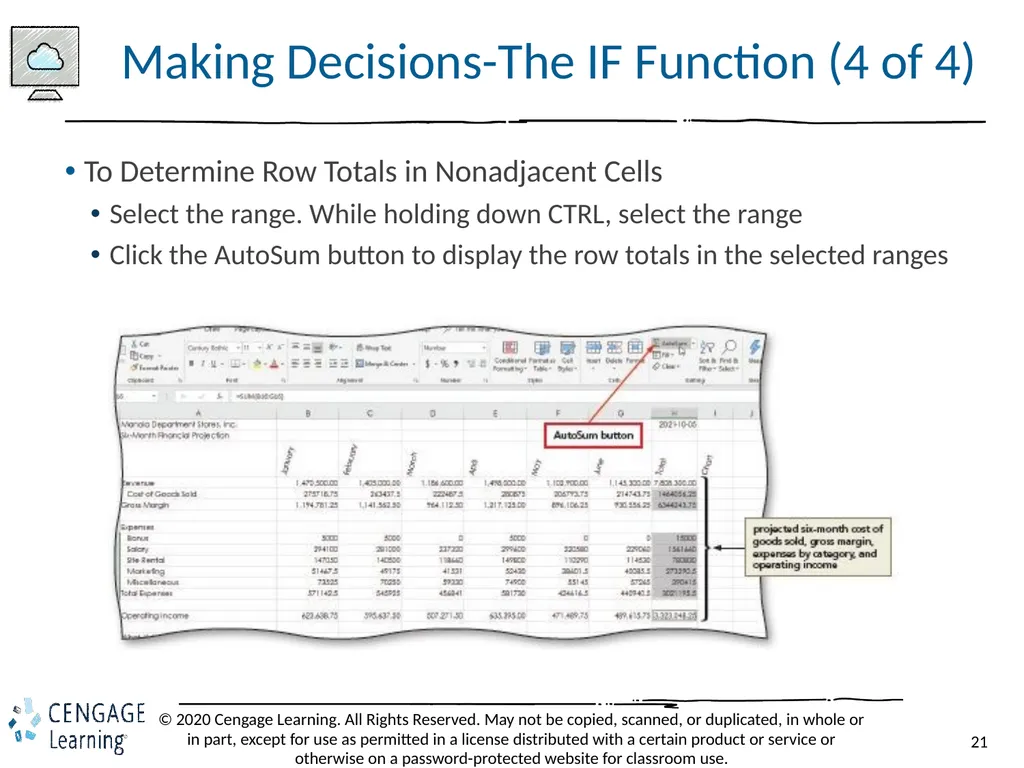
Making Decisions-The IF Function (4 of 4) To Determine Row Totals in Nonadjacent Cells
Select the range. While holding down CTRL, select the range
Click the AutoSum button to display the row totals in the selected ranges<br>
Select the range. While holding down CTRL, select the range
Click the AutoSum button to display the row totals in the selected ranges<br>
22
Adding and Formatting Sparkline Charts (1 of 4) To Add a Sparkline Chart to the Worksheet
Select the cell in which you want to insert a sparkline chart
Display the INSERT tab and then click the Line button to display the Create Sparklines dialog box
Drag through the range of cells of which you want to chart, and then lift your finger or release the mouse button to insert the selected range in the Data Range box
Click the OK button to insert a line sparkline chart in the selected cell and display the SPARKLINE TOOLS DESIGN tab<br>
Select the cell in which you want to insert a sparkline chart
Display the INSERT tab and then click the Line button to display the Create Sparklines dialog box
Drag through the range of cells of which you want to chart, and then lift your finger or release the mouse button to insert the selected range in the Data Range box
Click the OK button to insert a line sparkline chart in the selected cell and display the SPARKLINE TOOLS DESIGN tab<br>
23
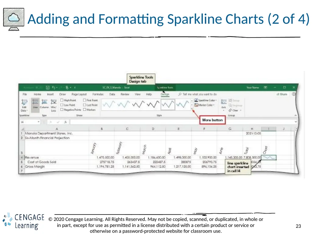
Adding and Formatting Sparkline Charts (2 of 4)<br>
24
Adding and Formatting Sparkline Charts (3 of 4) To Change the Sparkline Style and Copy the Sparkline Chart
Click the More button on the SPARKLINE TOOLS DESIGN tab to display the Sparkline Style gallery
Click a desired style in the Sparkline Style gallery to apply the style to the Sparkline chart in the selected cell
Point to the fill handle in the cell and then drag through the desired range to copy the line Sparkline chart<br>
Click the More button on the SPARKLINE TOOLS DESIGN tab to display the Sparkline Style gallery
Click a desired style in the Sparkline Style gallery to apply the style to the Sparkline chart in the selected cell
Point to the fill handle in the cell and then drag through the desired range to copy the line Sparkline chart<br>
25
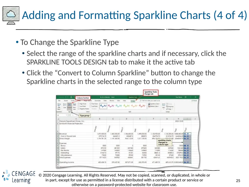
Adding and Formatting Sparkline Charts (4 of 4) To Change the Sparkline Type
Select the range of the sparkline charts and if necessary, click the SPARKLINE TOOLS DESIGN tab to make it the active tab
Click the “Convert to Column Sparkline” button to change the Sparkline charts in the selected range to the column type<br>
Select the range of the sparkline charts and if necessary, click the SPARKLINE TOOLS DESIGN tab to make it the active tab
Click the “Convert to Column Sparkline” button to change the Sparkline charts in the selected range to the column type<br>
26
Formatting the Worksheet (1 of 5) To Assign Formats to Nonadjacent Ranges
Select the first range to format
While holding down the CTRL key, select the nonadjacent ranges and then release the CTRL key to select nonadjacent ranges
Click the Number group on the HOME tab to display the Format Cells dialog box
Click the desired category and style, and then click the OK button<br>
Select the first range to format
While holding down the CTRL key, select the nonadjacent ranges and then release the CTRL key to select nonadjacent ranges
Click the Number group on the HOME tab to display the Format Cells dialog box
Click the desired category and style, and then click the OK button<br>
27
Formatting the Worksheet (2 of 5) To Format the Worksheet Titles
Press CTRL+HOME to select a cell and then click the column heading to select the column
Click the desired effect
Change font sizes
Change fill colors
Click empty cell to deselect the range<br>
Press CTRL+HOME to select a cell and then click the column heading to select the column
Click the desired effect
Change font sizes
Change fill colors
Click empty cell to deselect the range<br>
28
Formatting the Worksheet (3 of 5) To Assign Cell Styles to Nonadjacent Rows and Colors to a Cell
Select the range and apply a Heading style
Select a range and while holding down CTRL, select another range
Apply the Total cell style to the selected nonadjacent ranges
Select a cell and click Fill Color button on the HOME tab to apply the last fill color used to cell content
Click the Font Color button on the HOME tab to apply the last font color used<br>
Select the range and apply a Heading style
Select a range and while holding down CTRL, select another range
Apply the Total cell style to the selected nonadjacent ranges
Select a cell and click Fill Color button on the HOME tab to apply the last fill color used to cell content
Click the Font Color button on the HOME tab to apply the last font color used<br>
29
Formatting the Worksheet (4 of 5) To Copy a Cell’s Format Using the Format Painter Button
Select the source cell for the format to paint
Double-click the Format Painter button on the HOME tab and then move the pointer onto the worksheet to cause the pointer to change to a block plus sign with a paintbrush
Click the cell(s) to receive the format to assign the format of the source cell to the destination cell(s)
Click the Format Painter button or press the ESC key to stop the format painter<br>
Select the source cell for the format to paint
Double-click the Format Painter button on the HOME tab and then move the pointer onto the worksheet to cause the pointer to change to a block plus sign with a paintbrush
Click the cell(s) to receive the format to assign the format of the source cell to the destination cell(s)
Click the Format Painter button or press the ESC key to stop the format painter<br>
30
Formatting the Worksheet (5 of 5) To Format the What-If Assumptions Table
Select a cell
Change the font size
Italicize and underline the text
Select the range and change the font size, then click Fill Color button from the HOME tab to apply the most recently used background color to the selected range
Click the Font Color button on the HOME tab to apply the most recently used font color to the selected range
Deselect the range and display the What-IF Assumptions table
Save the workbook<br>
Select a cell
Change the font size
Italicize and underline the text
Select the range and change the font size, then click Fill Color button from the HOME tab to apply the most recently used background color to the selected range
Click the Font Color button on the HOME tab to apply the most recently used font color to the selected range
Deselect the range and display the What-IF Assumptions table
Save the workbook<br>
31
Adding a Clustered Column Chart to the Workbook (1 of 8) To Draw a Clustered Column Chart on a Separate Chart Sheet Using the Recommended Charts Features
Select a range to identify the range of the categories
Hold down the CTRL key and select a data range
Click the Recommended Charts button on the INSERT tab to display the Insert Chart dialog box with the Recommended Charts tab active
Click the recommended chart to select it and then click the OK button
When Excel draws the chart, click the Move Chart button on the CHART TOOLS DESIGN tab to display the Move Chart dialog box
Click New sheet and then enter a name in the in the New sheet text box to enter a sheet tab name for the chart sheet
Click the OK button to move the chart to a new chart sheet with a new sheet tab name<br>
Select a range to identify the range of the categories
Hold down the CTRL key and select a data range
Click the Recommended Charts button on the INSERT tab to display the Insert Chart dialog box with the Recommended Charts tab active
Click the recommended chart to select it and then click the OK button
When Excel draws the chart, click the Move Chart button on the CHART TOOLS DESIGN tab to display the Move Chart dialog box
Click New sheet and then enter a name in the in the New sheet text box to enter a sheet tab name for the chart sheet
Click the OK button to move the chart to a new chart sheet with a new sheet tab name<br>
32
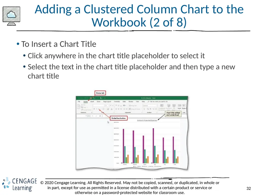
Adding a Clustered Column Chart to the Workbook (2 of 8) To Insert a Chart Title
Click anywhere in the chart title placeholder to select it
Select the text in the chart title placeholder and then type a new chart title<br>
Click anywhere in the chart title placeholder to select it
Select the text in the chart title placeholder and then type a new chart title<br>
33
Adding a Clustered Column Chart to the Workbook (3 of 8) To Add Data Labels
Click the Chart Elements button to display the CHART ELEMENTS gallery
Point to Data Labels to display an arrow and then click the arrow to display the Data Labels fly-out menu
Click a selection from the Data Labels fly-out menu so that data labels are displayed as desired
Click the Chart Elements button to close the gallery<br>
Click the Chart Elements button to display the CHART ELEMENTS gallery
Point to Data Labels to display an arrow and then click the arrow to display the Data Labels fly-out menu
Click a selection from the Data Labels fly-out menu so that data labels are displayed as desired
Click the Chart Elements button to close the gallery<br>
34
Adding a Clustered Column Chart to the Workbook (4 of 8) To Apply Chart Filters
Click the Chart Filters button (on the chart) to display the Chart Filters gallery
In the SERIES section, click the desired check boxes to remove their check marks and then click the Apply button to filter these series from the chart
Click the Chart Filters button to close the gallery<br>
Click the Chart Filters button (on the chart) to display the Chart Filters gallery
In the SERIES section, click the desired check boxes to remove their check marks and then click the Apply button to filter these series from the chart
Click the Chart Filters button to close the gallery<br>
35
Adding a Clustered Column Chart to the Workbook (5 of 8) To Add an Axis Title to the Chart
Click anywhere in the chart area outside the chart to select the chart, and then click the Chart Elements button to display the CHART ELEMENTS gallery
Point to Axis Titles to display an arrow and then click the arrow to display the Axis Titles fly-out menu
Click an axis on the Axis Titles fly-out menu to add an axis title, and then click the Chart Elements button to remove the CHART ELEMENTS gallery
Select the placeholder text in the axis title and replace it with the desired text
Right-click the axis title to display a shortcut menu, and then click “Format Axis Title” on the shortcut menu to open the Format Axis Title task pane
Click the TITLE OPTIONS tab, click the “Size & Properties” button, and then, if necessary, click the ALIGNMENT arrow to expand the ALIGNMENT section
Click the Text direction arrow, and then click the desired direction from the direction list to change the orientation of the axis title<br>
Click anywhere in the chart area outside the chart to select the chart, and then click the Chart Elements button to display the CHART ELEMENTS gallery
Point to Axis Titles to display an arrow and then click the arrow to display the Axis Titles fly-out menu
Click an axis on the Axis Titles fly-out menu to add an axis title, and then click the Chart Elements button to remove the CHART ELEMENTS gallery
Select the placeholder text in the axis title and replace it with the desired text
Right-click the axis title to display a shortcut menu, and then click “Format Axis Title” on the shortcut menu to open the Format Axis Title task pane
Click the TITLE OPTIONS tab, click the “Size & Properties” button, and then, if necessary, click the ALIGNMENT arrow to expand the ALIGNMENT section
Click the Text direction arrow, and then click the desired direction from the direction list to change the orientation of the axis title<br>
36
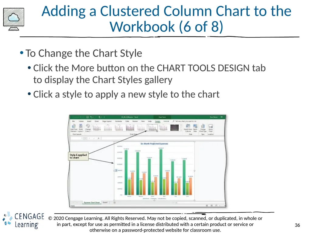
Adding a Clustered Column Chart to the Workbook (6 of 8) To Change the Chart Style
Click the More button on the CHART TOOLS DESIGN tab to display the Chart Styles gallery
Click a style to apply a new style to the chart<br>
Click the More button on the CHART TOOLS DESIGN tab to display the Chart Styles gallery
Click a style to apply a new style to the chart<br>
37
Adding a Clustered Column Chart to the Workbook (7 of 8) To Modify the Chart Axis Number Format
Right-click any value on the vertical axis to display the shortcut menu, and then click Format Axis to open the Format Axis task pane
If necessary, click the AXIS OPTIONS tab and then scroll until NUMBER is visible
Click the NUMBER arrow to expand the NUMBER section and then scroll to display options related to formatting numbers
Change the number to the desired format<br>
Right-click any value on the vertical axis to display the shortcut menu, and then click Format Axis to open the Format Axis task pane
If necessary, click the AXIS OPTIONS tab and then scroll until NUMBER is visible
Click the NUMBER arrow to expand the NUMBER section and then scroll to display options related to formatting numbers
Change the number to the desired format<br>
38
Adding a Clustered Column Chart to the Workbook (8 of 8) To Remove Filters and Data Labels
Click the CHART ELEMENTS button to display the Chart Elements gallery
Click the Data Labels check box to remove the check mark for the data labels
Click the CHART ELEMENTS button again to close the gallery
Click the CHART FILTERS button to display the Chart Filters fly-out menu
In the Series section, click desired series, click APPLY button to add the series back into the chart and then click the CHART FILTERS button again to close the menu<br>
Click the CHART ELEMENTS button to display the Chart Elements gallery
Click the Data Labels check box to remove the check mark for the data labels
Click the CHART ELEMENTS button again to close the gallery
Click the CHART FILTERS button to display the Chart Filters fly-out menu
In the Series section, click desired series, click APPLY button to add the series back into the chart and then click the CHART FILTERS button again to close the menu<br>
39
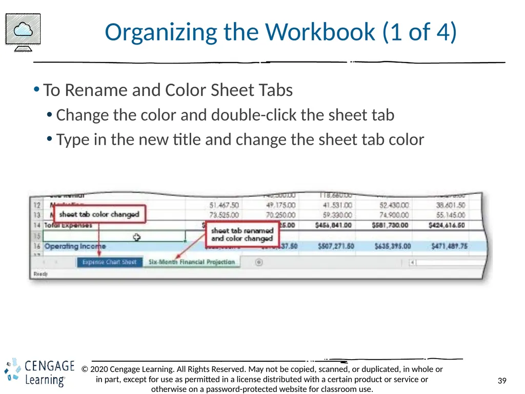
Organizing the Workbook (1 of 4) To Rename and Color Sheet Tabs
Change the color and double-click the sheet tab
Type in the new title and change the sheet tab color<br>
Change the color and double-click the sheet tab
Type in the new title and change the sheet tab color<br>
40
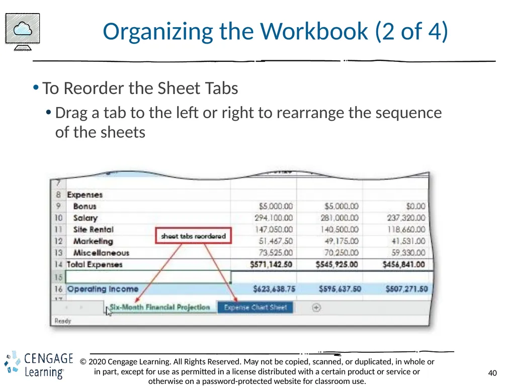
Organizing the Workbook (2 of 4) To Reorder the Sheet Tabs
Drag a tab to the left or right to rearrange the sequence of the sheets<br>
Drag a tab to the left or right to rearrange the sequence of the sheets<br>
41
Organizing the Workbook (3 of 4) To Check Spelling in Multiple Sheets
With the selected sheet active, press CTRL+HOME to select cell A1. Hold down CTRL and then click the selected tab to select both sheets
Display the REVIEW tab and click the Spelling button to check spelling.
Correct and errors and then click OK<br>
With the selected sheet active, press CTRL+HOME to select cell A1. Hold down CTRL and then click the selected tab to select both sheets
Display the REVIEW tab and click the Spelling button to check spelling.
Correct and errors and then click OK<br>
42
Organizing the Workbook (4 of 4) To Preview and Print the Worksheet
Click File on the ribbon to display the Print screen
Click Portrait Orientation button in the Settings area and then select Landscape Orientation
Click the No Scaling button and then select “Fit Sheet on One page”
Verify the desired printer is selected
Click Print<br>
Click File on the ribbon to display the Print screen
Click Portrait Orientation button in the Settings area and then select Landscape Orientation
Click the No Scaling button and then select “Fit Sheet on One page”
Verify the desired printer is selected
Click Print<br>
43
Changing the View of the Worksheet (1 of 4) To Shrink and Magnify the View of a Worksheet or Chart
Display the VIEW tab and then click the Zoom button to display a list of magnifications in the Zoom dialog box
Click the desired zoom level, and then click the OK button
Click the Zoom in button on the status bar until the worksheet is displayed at the desired magnification<br>
Display the VIEW tab and then click the Zoom button to display a list of magnifications in the Zoom dialog box
Click the desired zoom level, and then click the OK button
Click the Zoom in button on the status bar until the worksheet is displayed at the desired magnification<br>
44
Changing the View of the Worksheet (2 of 4) To Split a Window into Panes
Click the cell at the intersection of the four proposed panes to select the cell at which to split the window
Click the Split button on the VIEW tab to divide the window into four panes
To Remove the Panes from the Window
Click the SPLIT button to remove the four panes from the window<br>
Click the cell at the intersection of the four proposed panes to select the cell at which to split the window
Click the Split button on the VIEW tab to divide the window into four panes
To Remove the Panes from the Window
Click the SPLIT button to remove the four panes from the window<br>
45
Changing the View of the Worksheet (3 of 4) To Freeze Worksheet Columns and Rows
Click the cell at the intersection of the row and column at which to freeze panes
Click the Freeze Panes button on the VIEW tab to display the Freeze Panes gallery
Click Freeze Panes in the Freeze Panes gallery to freeze rows and columns to the left and above the selected cell<br>
Click the cell at the intersection of the row and column at which to freeze panes
Click the Freeze Panes button on the VIEW tab to display the Freeze Panes gallery
Click Freeze Panes in the Freeze Panes gallery to freeze rows and columns to the left and above the selected cell<br>
46
Changing the View of the Worksheet (4 of 4) To Unfreeze Worksheet Columns and Rows
Press CTRL+HOME to select a cell and view the supper-left corner of the screen
Click the Freeze Panes button on the VIEW tab to display the Freeze Panes gallery
Click Unfreeze Panes in the Freeze Panes gallery to unfreeze the frozen columns and rows<br>
Press CTRL+HOME to select a cell and view the supper-left corner of the screen
Click the Freeze Panes button on the VIEW tab to display the Freeze Panes gallery
Click Unfreeze Panes in the Freeze Panes gallery to unfreeze the frozen columns and rows<br>
47
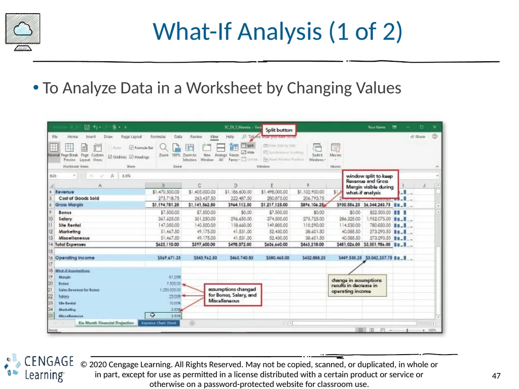
What-If Analysis (1 of 2) To Analyze Data in a Worksheet by Changing Values<br>
48
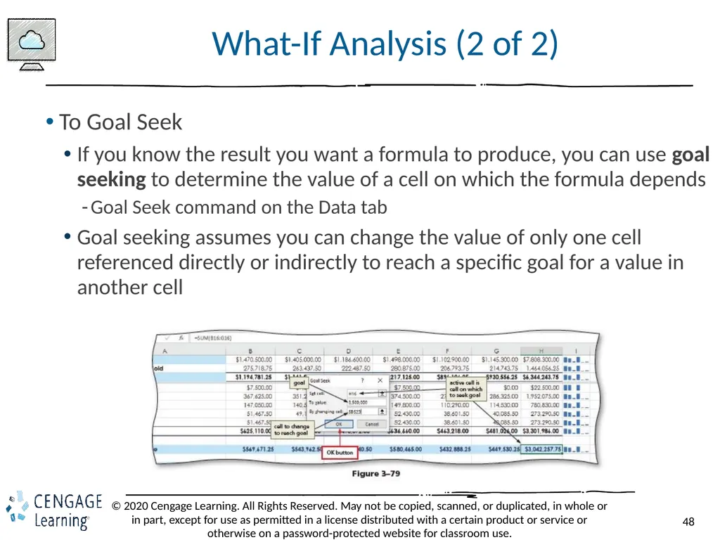
What-If Analysis (2 of 2) To Goal Seek
If you know the result you want a formula to produce, you can use goal seeking to determine the value of a cell on which the formula depends
Goal Seek command on the Data tab
Goal seeking assumes you can change the value of only one cell referenced directly or indirectly to reach a specific goal for a value in another cell<br>
If you know the result you want a formula to produce, you can use goal seeking to determine the value of a cell on which the formula depends
Goal Seek command on the Data tab
Goal seeking assumes you can change the value of only one cell referenced directly or indirectly to reach a specific goal for a value in another cell<br>
49
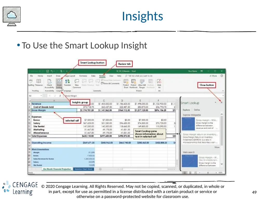
Insights To Use the Smart Lookup Insight<br>
50
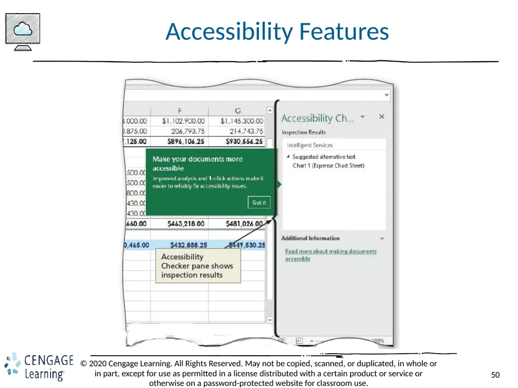
Accessibility Features<br>