Survival analysis using Stata Gabriela Ortiz 1
Description: Survival analysis using Stata Gabriela Ortiz 1 Overview Introduction to survival-time data Summary statistics Exploratory graphs Estimation Semiparametric and parametric models Predictions Diagnostics Goodness-of-fit plots Testing
Related Topics
Download Presentation
"Survival analysis using Stata Gabriela Ortiz 1" is the property of its rightful owner. Permission is granted to download and print the materials on this website for personal, non-commercial use only, and to display it on your personal computer provided you do not modify the materials and that you retain all copyright notices contained in the materials. By downloading content from our website, you accept the terms of this agreement.
Presentation Transcript
slide1. Survival analysis using Stata Gabriela Ortiz 1<br>
slide2. Overview Introduction to survival-time data
Summary statistics
Exploratory graphs
Estimation
Semiparametric and parametric models
Predictions
Diagnostics
Goodness-of-fit plots
Testing assumptions 2<br>
slide3. Introduction to survival data 3<br>
slide4. Survival-time data We measure time to an event of interest
The occurrence of the event is typically called a failure
An observation is censored if we don’t know the exact time of failure
Survival-time data is present in many fields
Health
Economics
Business
Criminology
Stata’s st suite of commands is designed for analyzing survival-time data 4<br>
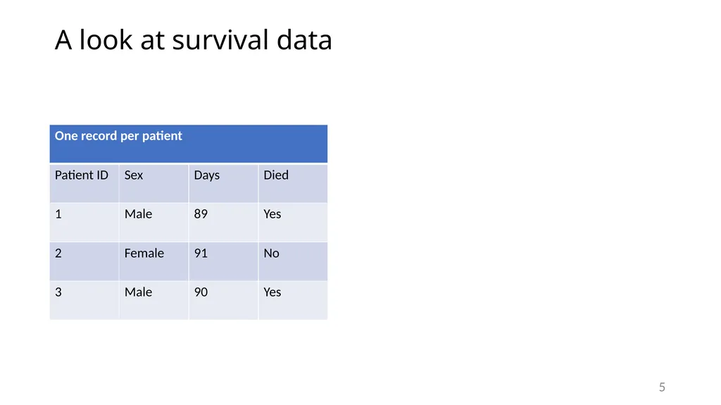
slide5. A look at survival data 5<br>
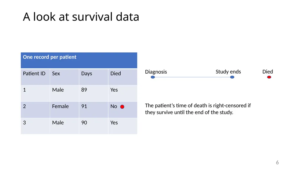
slide6. A look at survival data 6 Diagnosis Study ends The patient’s time of death is right-censored if they survive until the end of the study. Died<br>
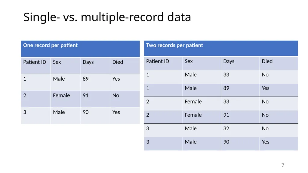
slide7. Single- vs. multiple-record data 7<br>
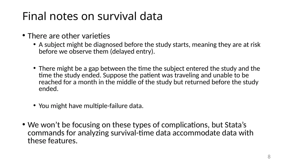
slide8. Final notes on survival data There are other varieties
A subject might be diagnosed before the study starts, meaning they are at risk before we observe them (delayed entry).
There might be a gap between the time the subject entered the study and the time the study ended. Suppose the patient was traveling and unable to be reached for a month in the middle of the study but returned before the study ended.
You might have multiple-failure data.
We won’t be focusing on these types of complications, but Stata’s commands for analyzing survival-time data accommodate data with these features. 8<br>
slide9. A first example 9<br>
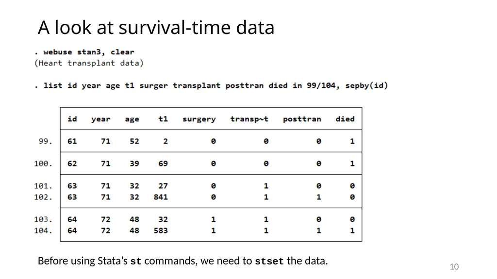
slide10. A look at survival-time data Before using Stata’s st commands, we need to stset the data. 10<br>
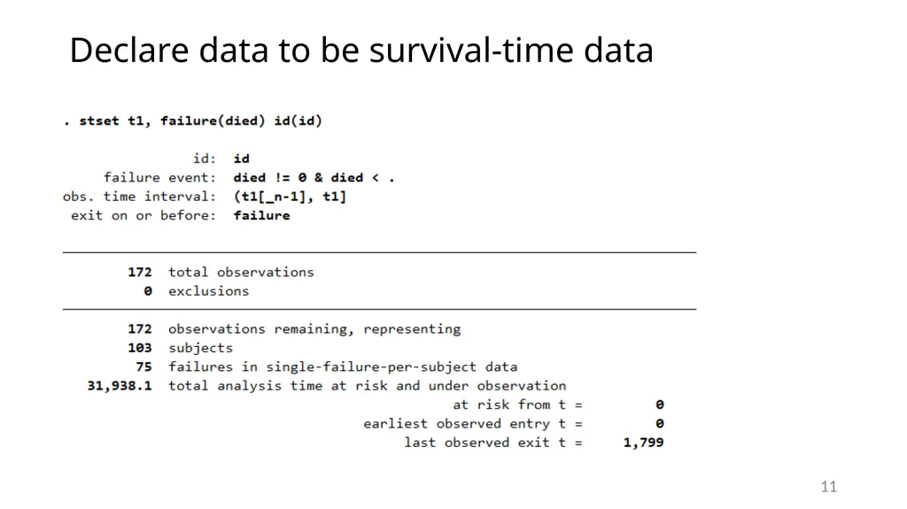
slide11. Declare data to be survival-time data 11<br>
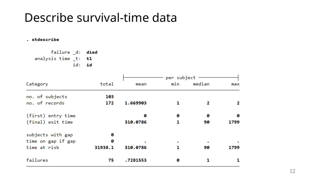
slide12. Describe survival-time data 12<br>
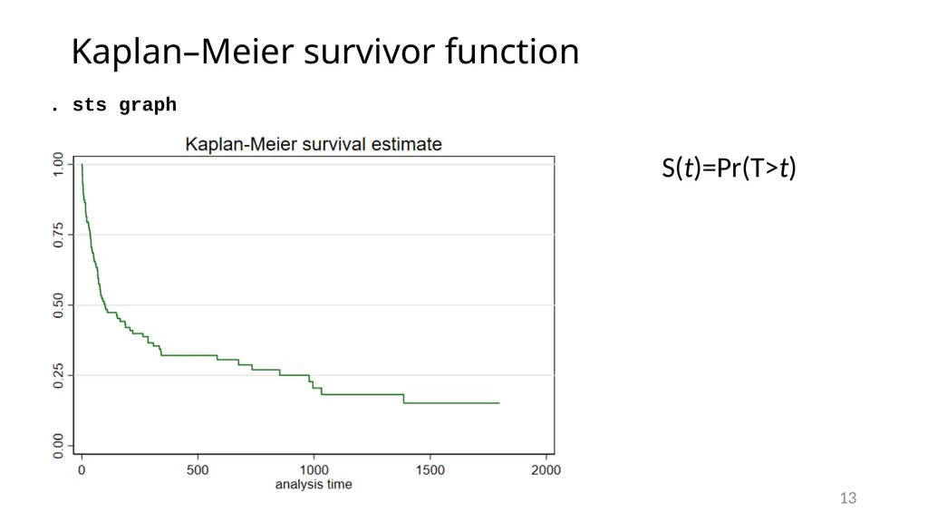
slide13. Kaplan–Meier survivor function 13 . sts graph S(t)=Pr(T>t)<br>
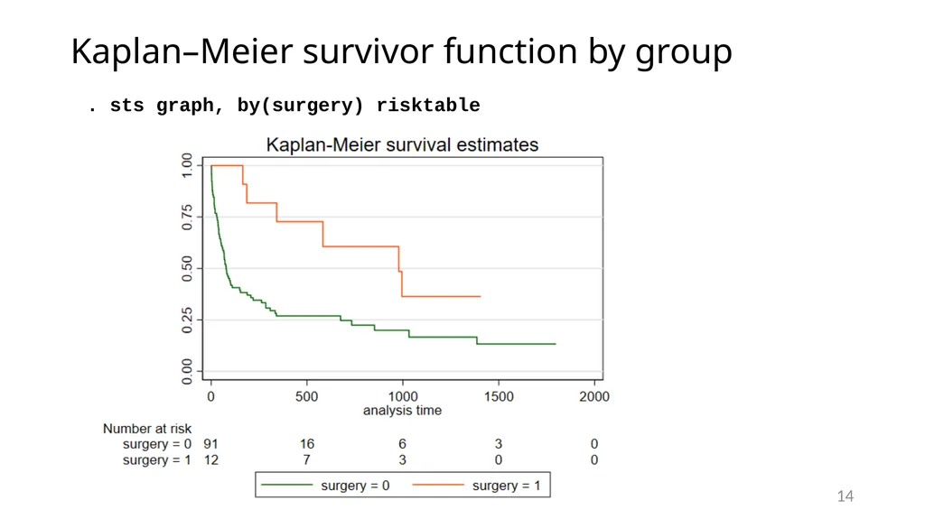
slide14. Kaplan–Meier survivor function by group 14 . sts graph, by(surgery) risktable<br>
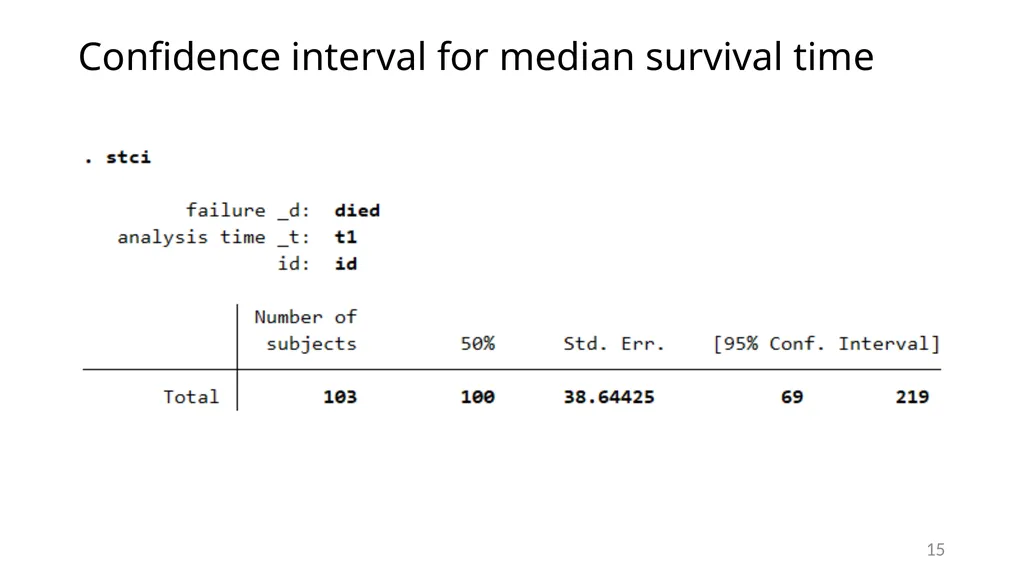
slide15. Confidence interval for median survival time 15<br>
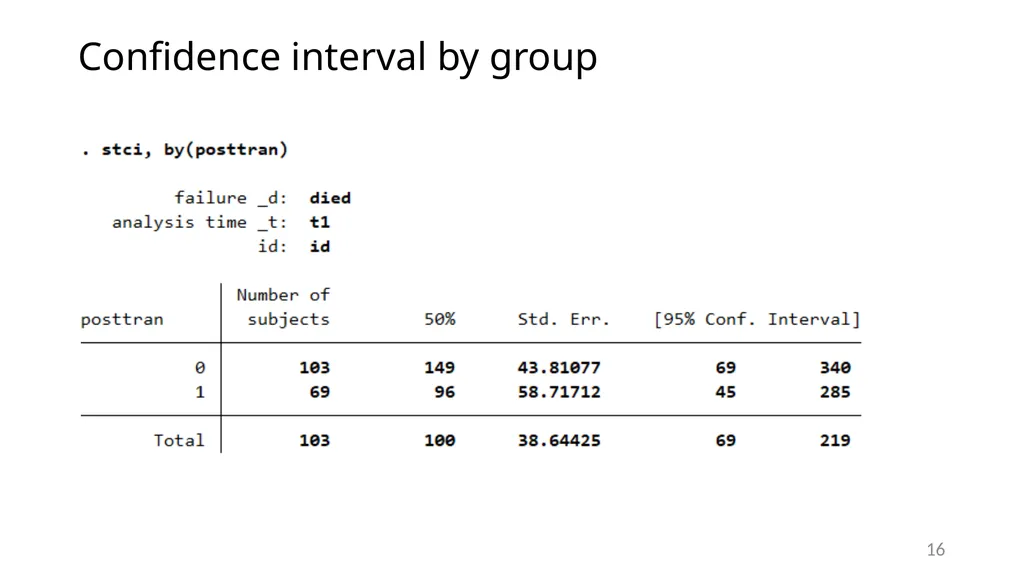
slide16. Confidence interval by group 16<br>
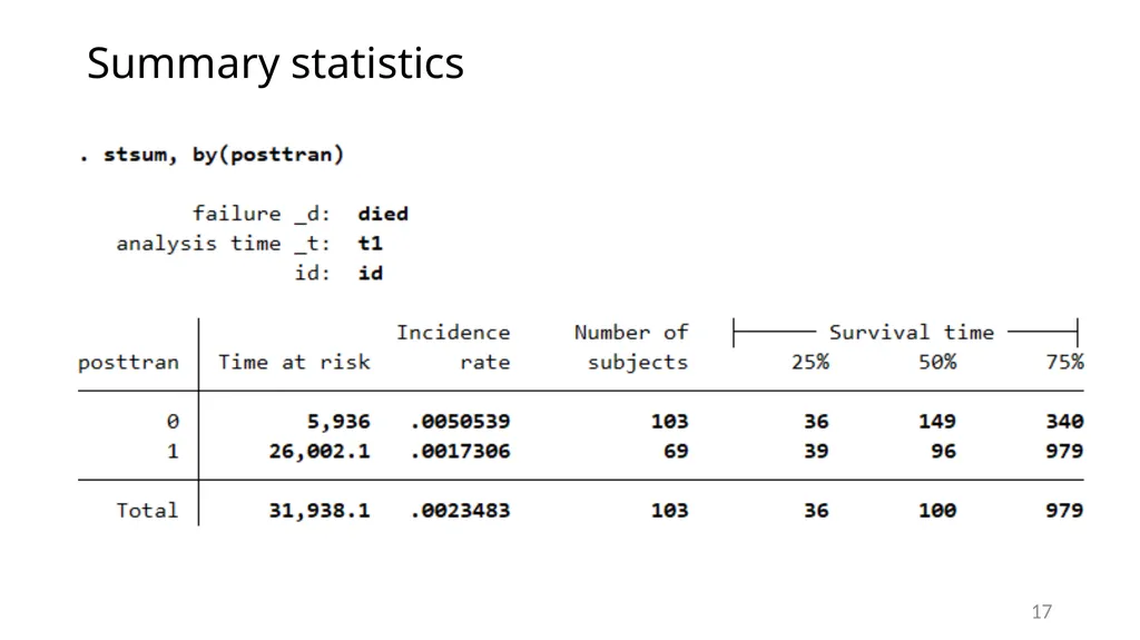
slide17. Summary statistics 17<br>
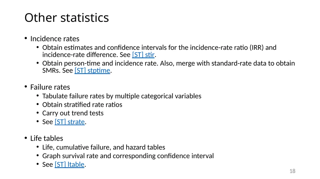
slide18. Other statistics Incidence rates
Obtain estimates and confidence intervals for the incidence-rate ratio (IRR) and incidence-rate difference. See [ST] stir.
Obtain person-time and incidence rate. Also, merge with standard-rate data to obtain SMRs. See [ST] stptime.
Failure rates
Tabulate failure rates by multiple categorical variables
Obtain stratified rate ratios
Carry out trend tests
See [ST] strate.
Life tables
Life, cumulative failure, and hazard tables
Graph survival rate and corresponding confidence interval
See [ST] ltable. 18<br>
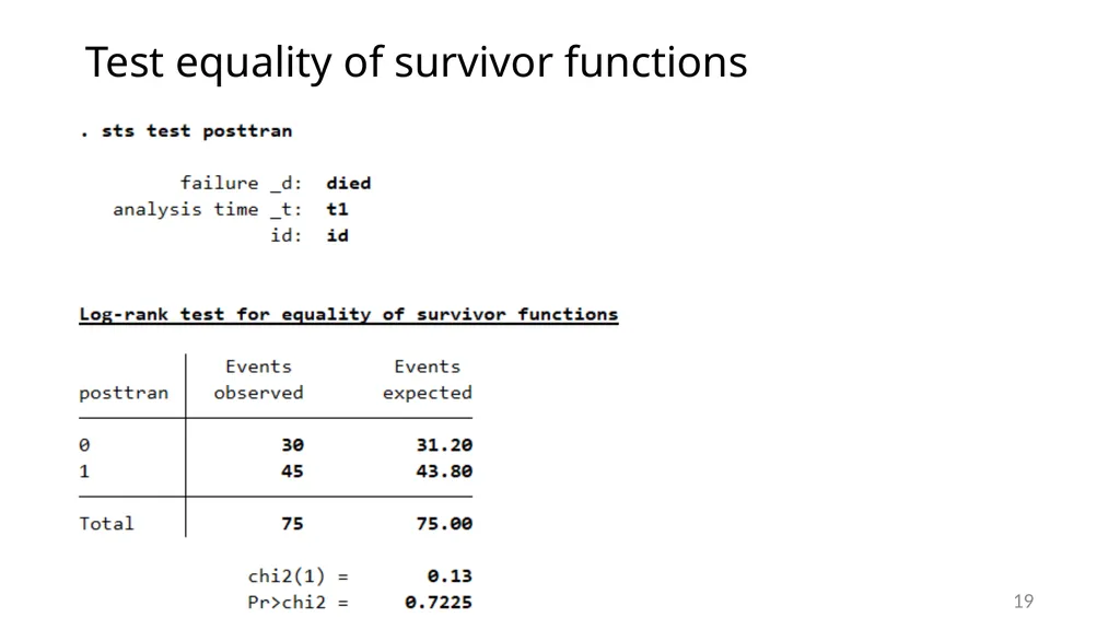
slide19. Test equality of survivor functions 19<br>
slide20. Cox proportional hazards model 20<br>
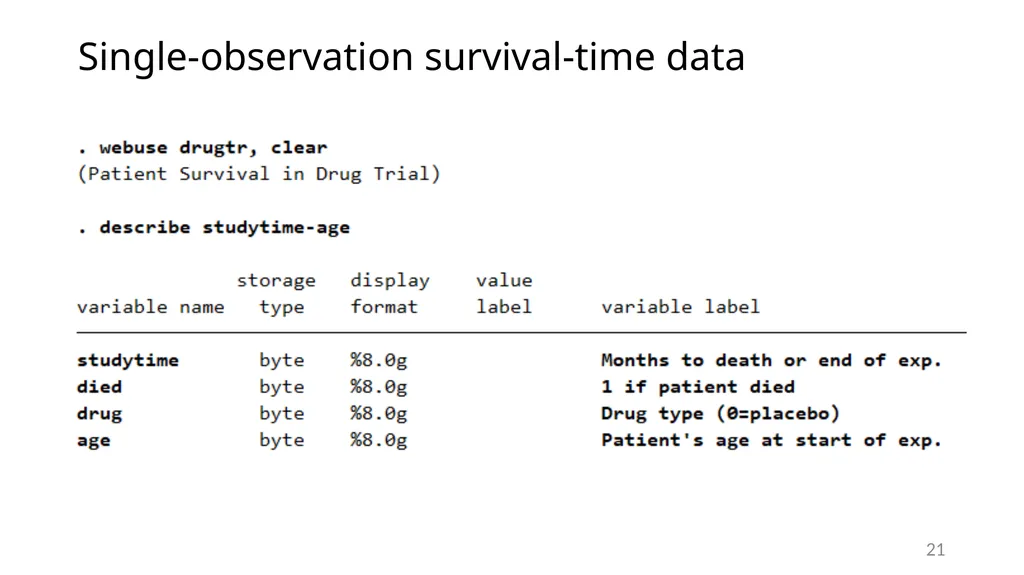
slide21. Single-observation survival-time data 21<br>
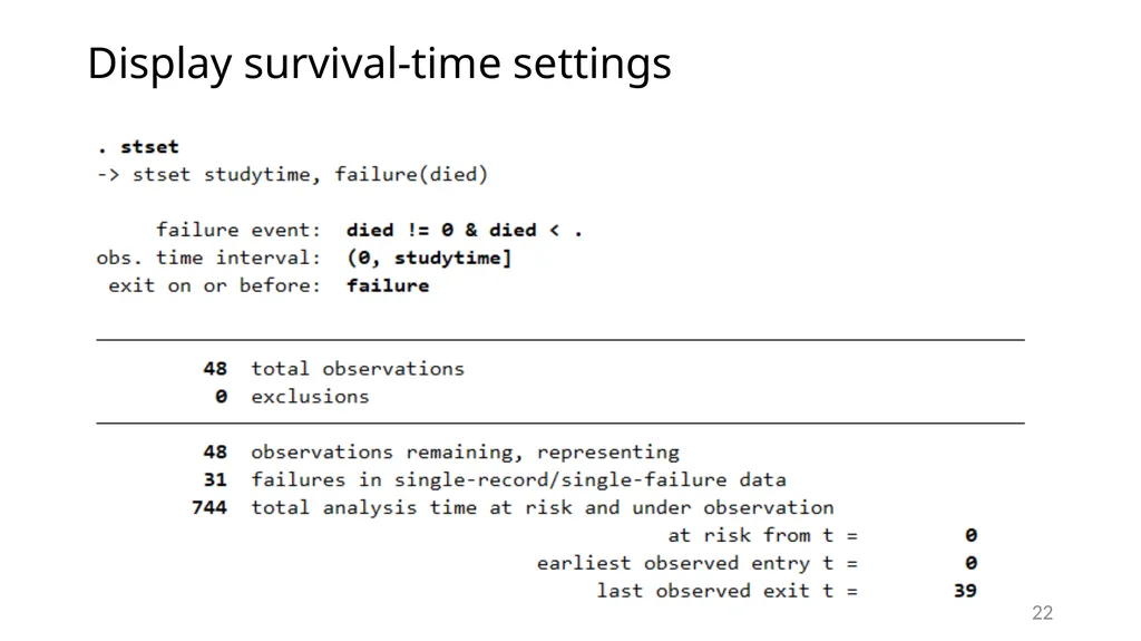
slide22. Display survival-time settings 22<br>
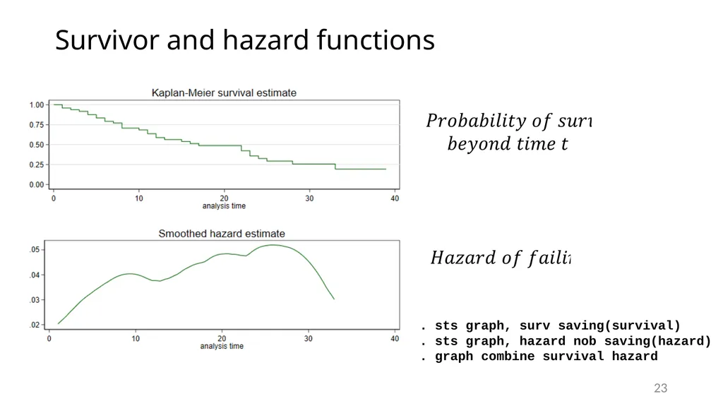
slide23. Survivor and hazard functions 23 . sts graph, surv saving(survival)
. sts graph, hazard nob saving(hazard)
. graph combine survival hazard<br>
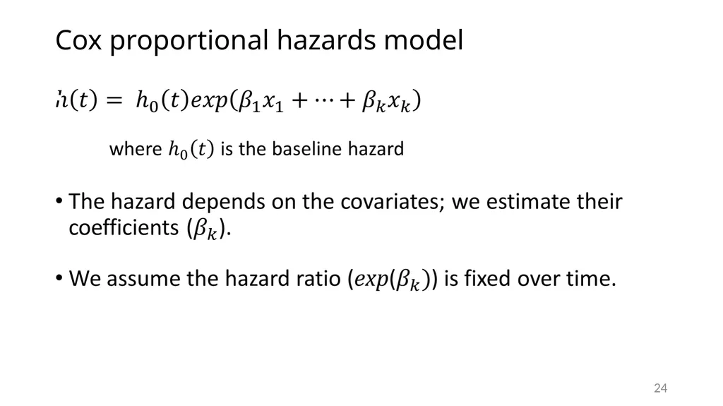
slide24. Cox proportional hazards model 24<br>
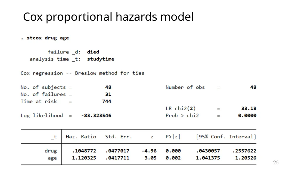
slide25. Cox proportional hazards model 25<br>
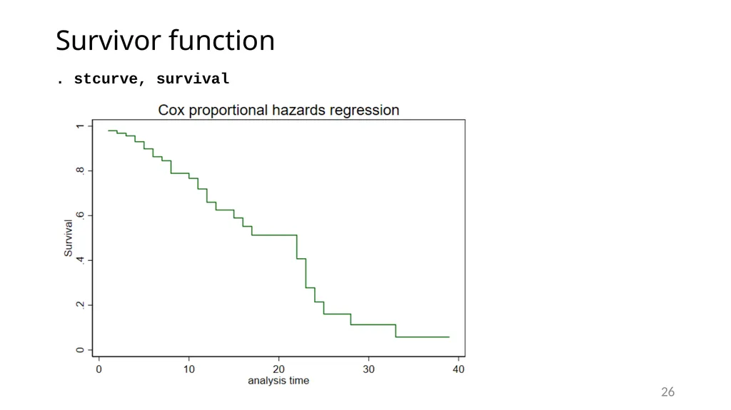
slide26. Survivor function 26 . stcurve, survival<br>
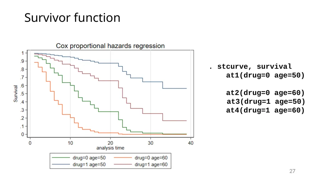
slide27. Survivor function 27 . stcurve, survival
at1(drug=0 age=50)
at2(drug=0 age=60)
at3(drug=1 age=50)
at4(drug=1 age=60)<br>
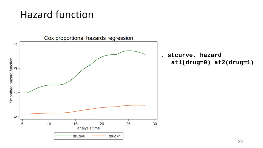
slide28. Hazard function 28 . stcurve, hazard
at1(drug=0) at2(drug=1)<br>
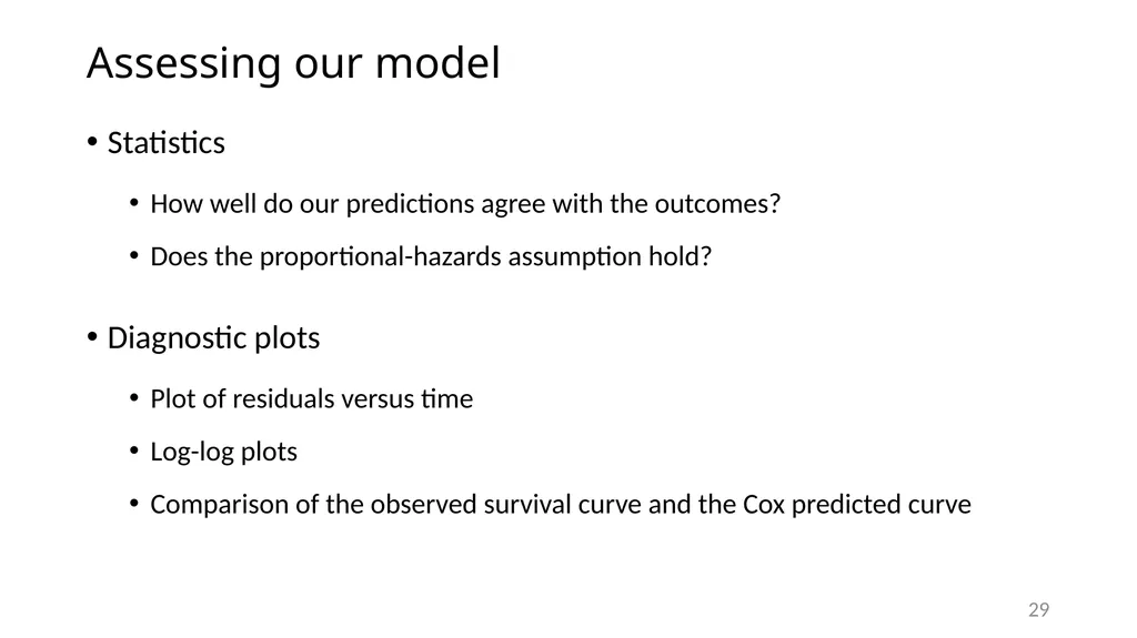
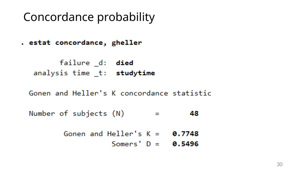
slide29. Assessing our model Statistics
How well do our predictions agree with the outcomes?
Does the proportional-hazards assumption hold?
Diagnostic plots
Plot of residuals versus time
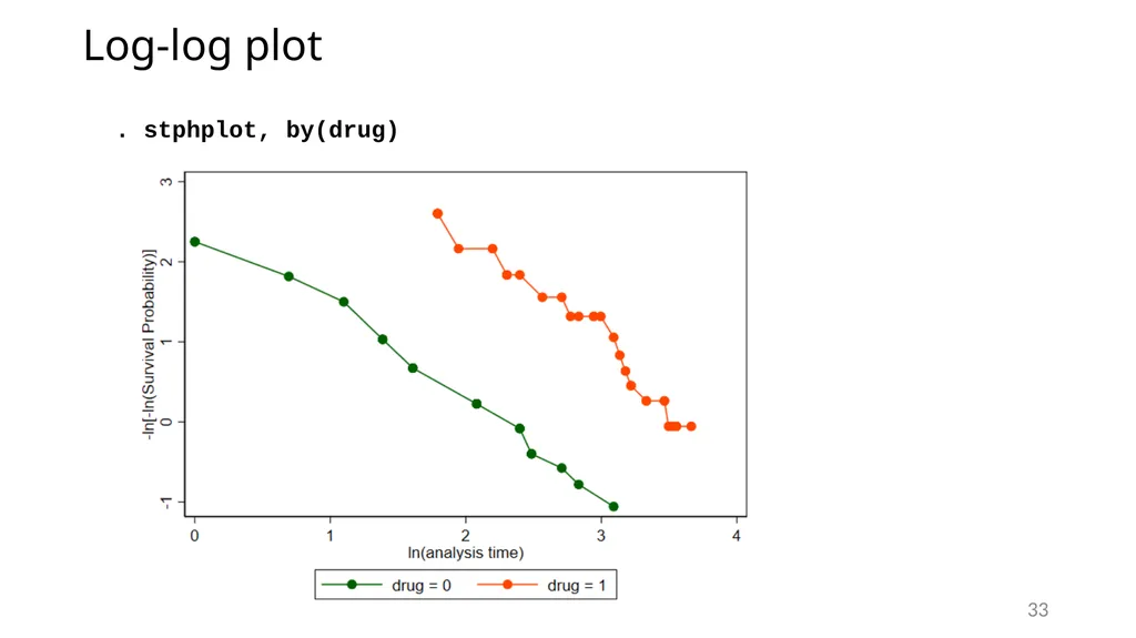
Log-log plots
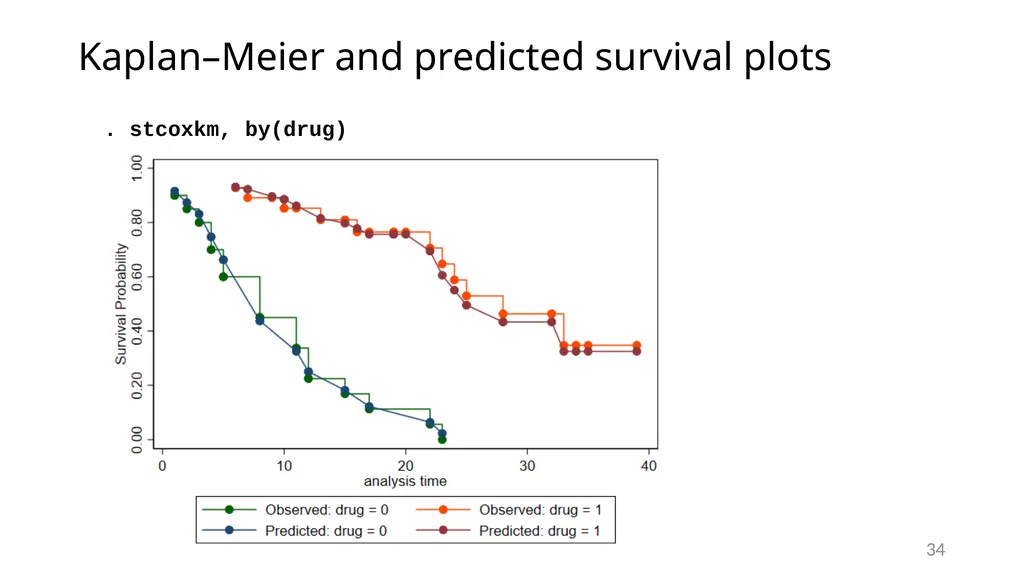
Comparison of the observed survival curve and the Cox predicted curve 29<br>
slide30. Concordance probability 30<br>
slide31. Test the proportional hazards assumption 31<br>
slide32. Plotting Schoenfeld residuals versus time 32 . estat phtest, plot(drug)<br>
slide33. . stphplot, by(drug) Log-log plot 33<br>
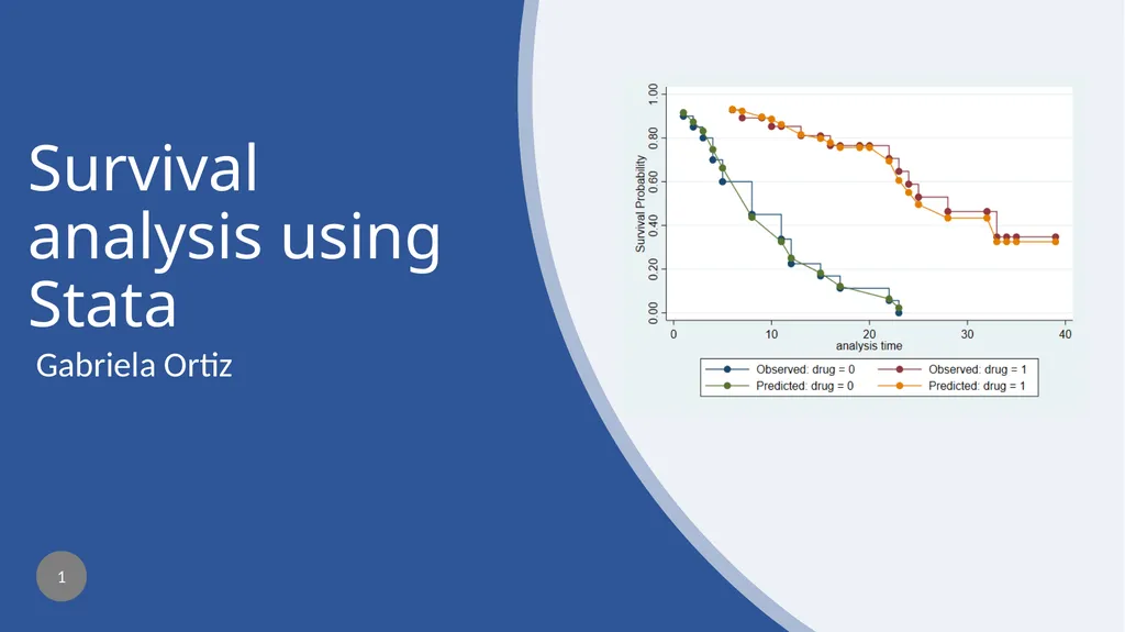
slide34. . stcoxkm, by(drug) Kaplan–Meier and predicted survival plots 34<br>
slide35. More on the proportional-hazards assumption Graphical assessment of the proportional-hazards assumption
Log-log plots
Adjust the estimates to average values of specified variables
Kaplan–Meier and predicted survival plots
Specify the method to handle tied failures
Test the proportional-hazards assumption
Test using Schoenfeld residuals
Choose from other time-scale functions or specify your own function of time
To learn more, see [ST]stcox PH-assumption tests. 35<br>
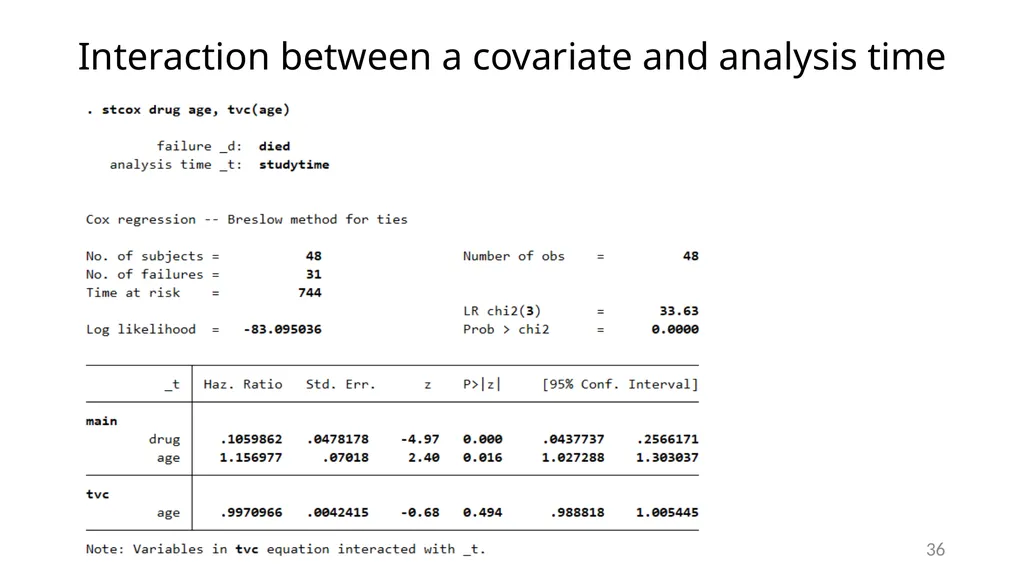
slide36. Interaction between a covariate and analysis time 36<br>
slide37. Shared-frailty models 37<br>
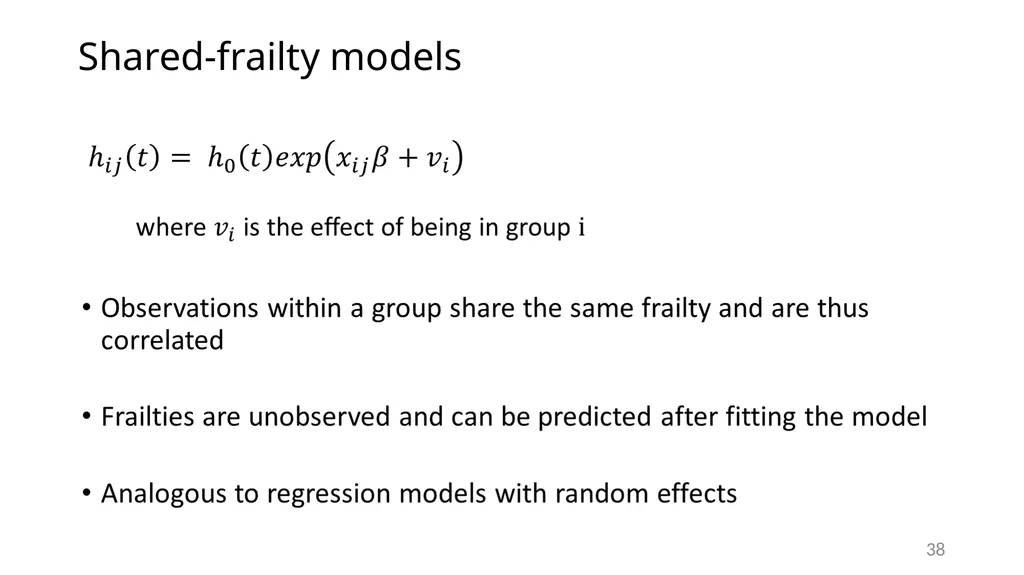
slide38. Shared-frailty models 38<br>
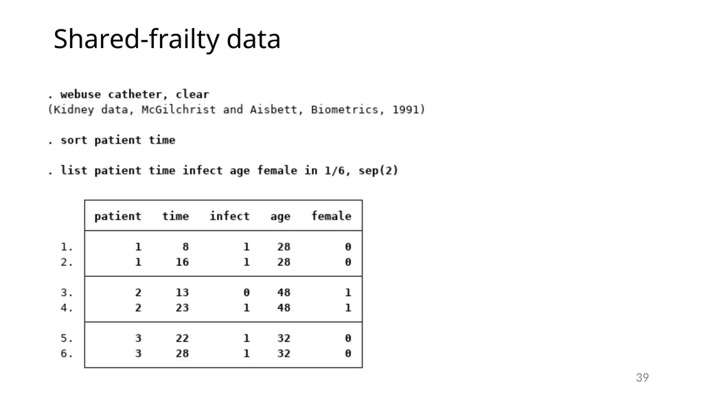
slide39. Shared-frailty data 39<br>
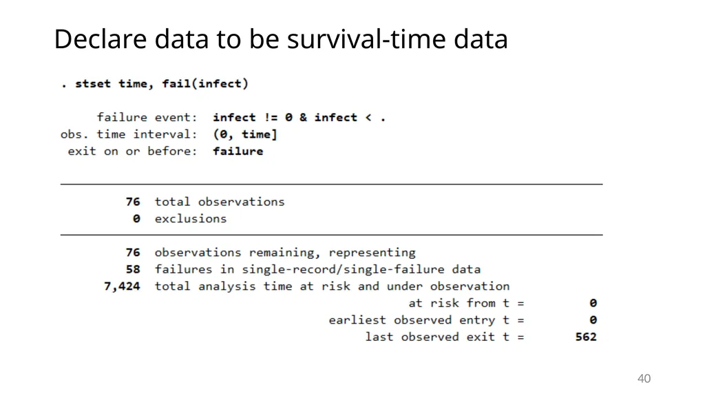
slide40. Declare data to be survival-time data 40<br>
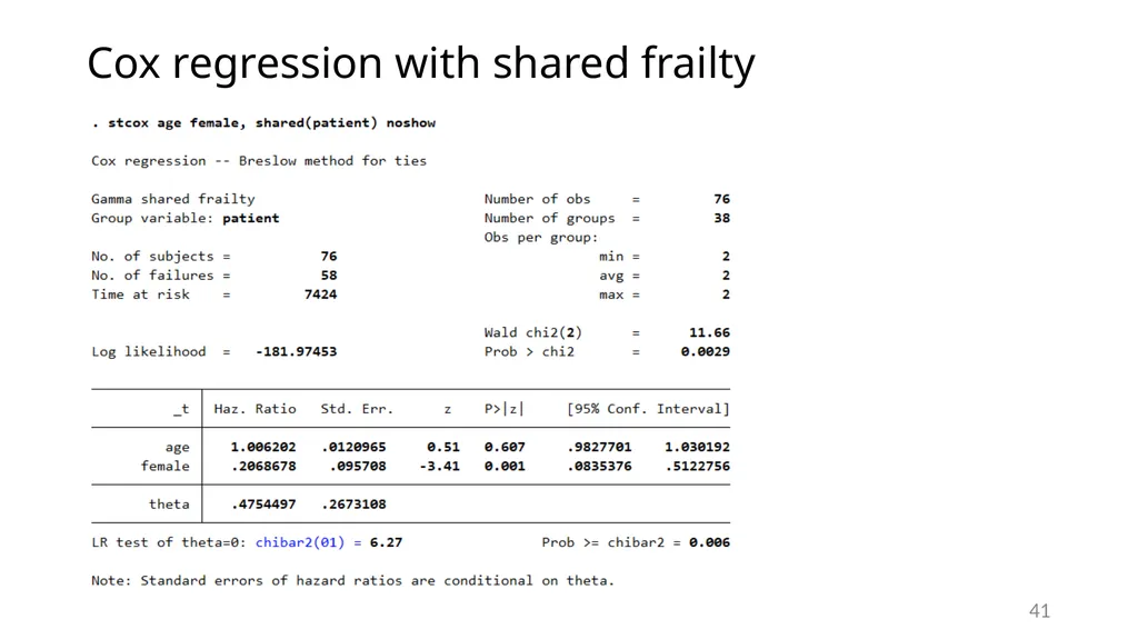
slide41. Cox regression with shared frailty 41<br>
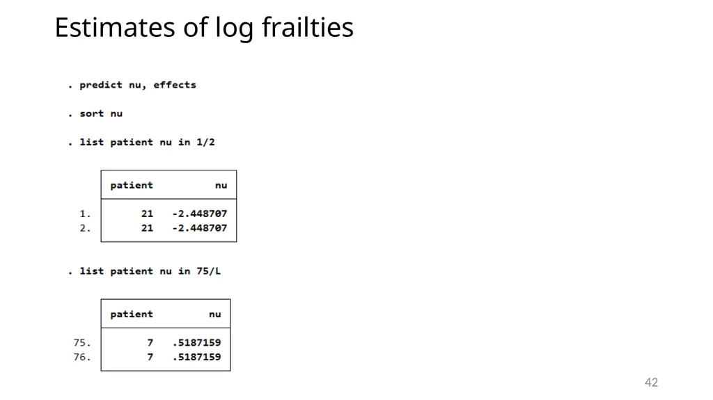
slide42. Estimates of log frailties 42<br>
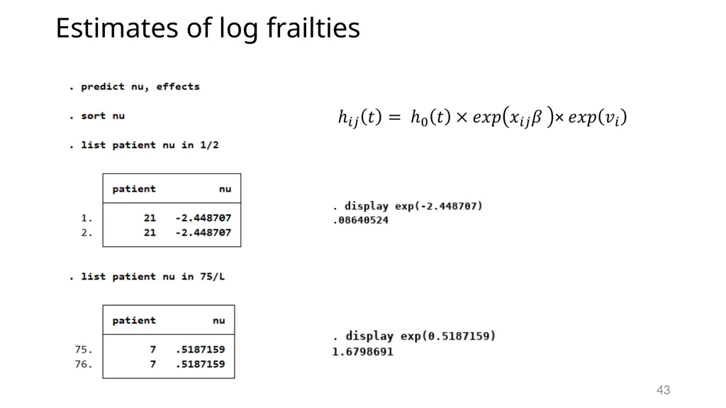
slide43. Estimates of log frailties 43<br>
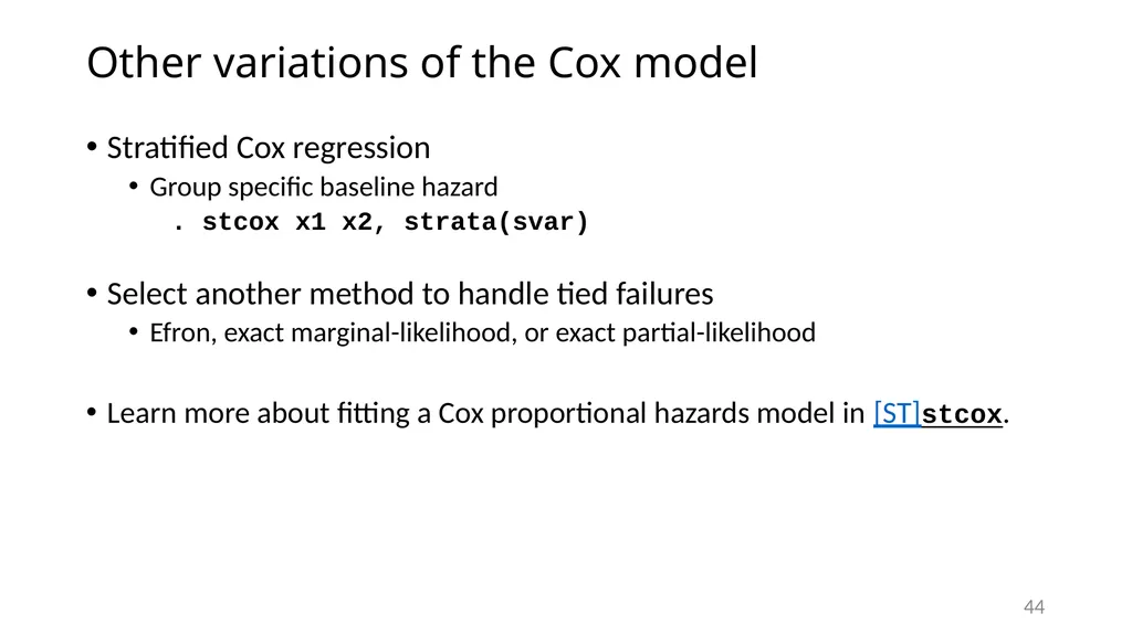
slide44. Other variations of the Cox model Stratified Cox regression
Group specific baseline hazard
. stcox x1 x2, strata(svar)
Select another method to handle tied failures
Efron, exact marginal-likelihood, or exact partial-likelihood
Learn more about fitting a Cox proportional hazards model in [ST]stcox. 44<br>
slide45. Competing risks regression models 45<br>
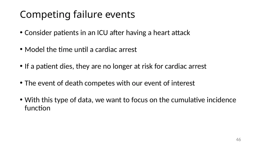
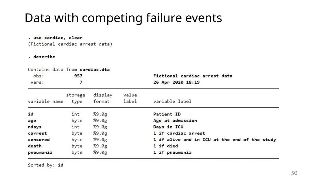
slide46. Competing failure events Consider patients in an ICU after having a heart attack
Model the time until a cardiac arrest
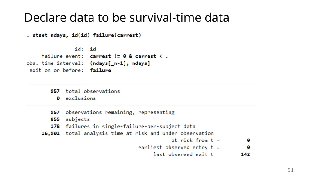
If a patient dies, they are no longer at risk for cardiac arrest
The event of death competes with our event of interest
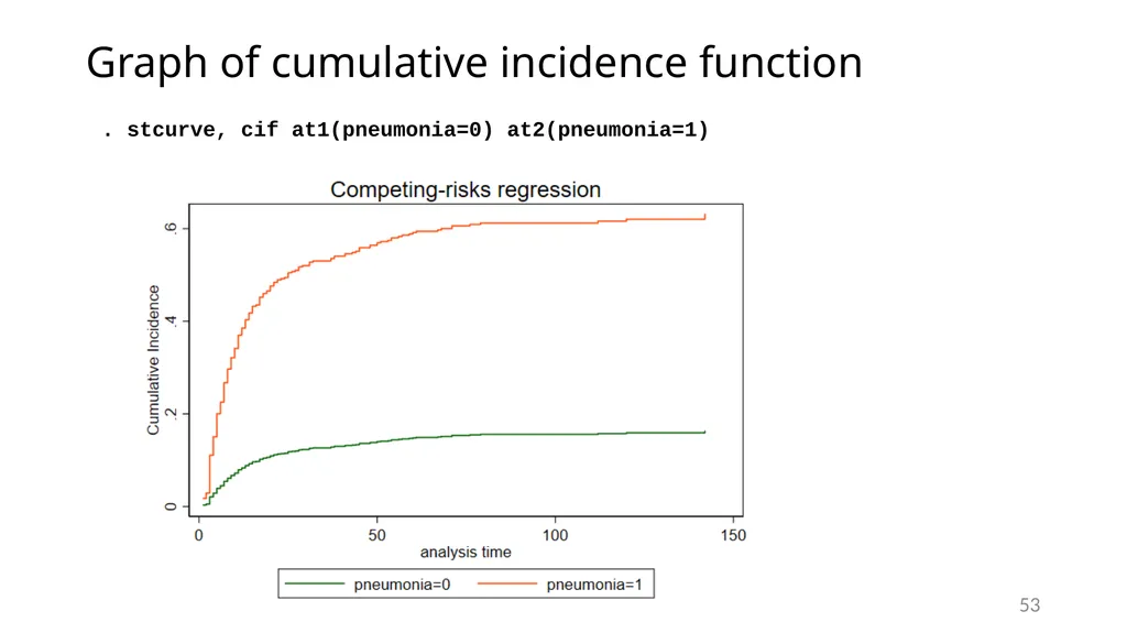
With this type of data, we want to focus on the cumulative incidence function 46<br>
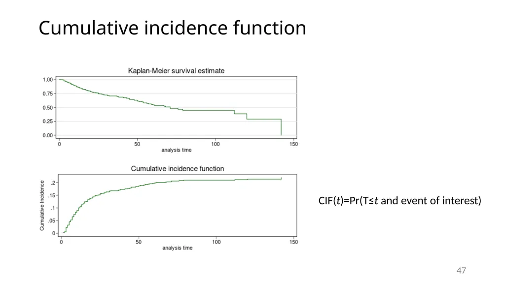
slide47. Cumulative incidence function 47 CIF(t)=Pr(T≤t and event of interest)<br>
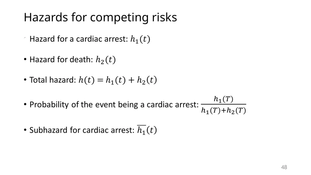
slide48. Hazards for competing risks 48<br>
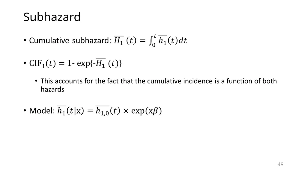
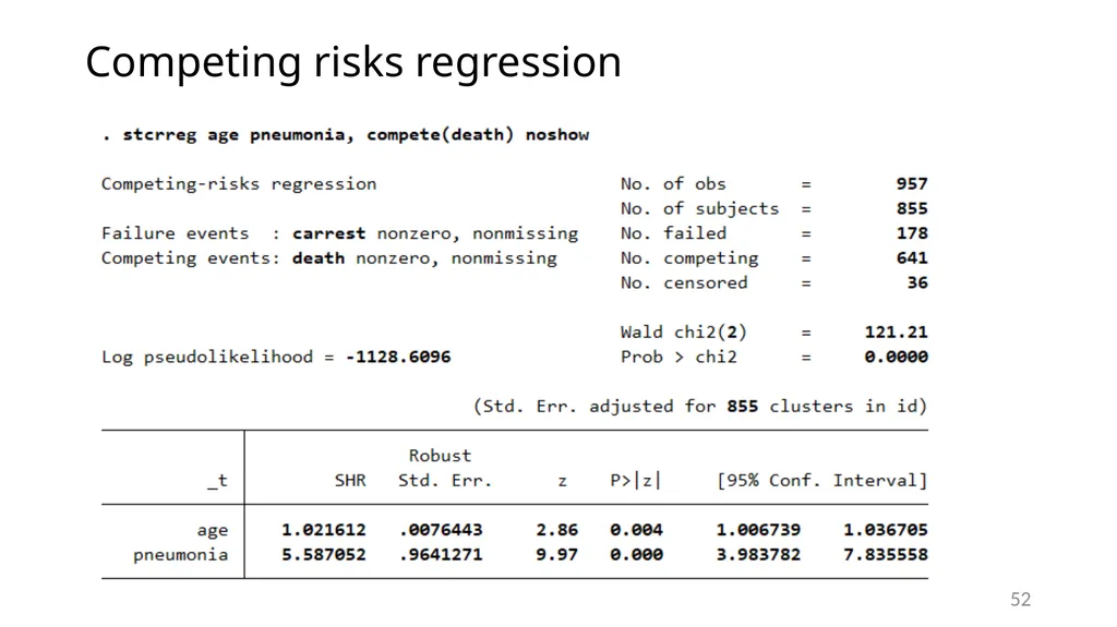
slide49. Subhazard 49<br>
slide50. Data with competing failure events 50<br>
slide51. Declare data to be survival-time data 51<br>
slide52. Competing risks regression 52<br>
slide53. Graph of cumulative incidence function 53 . stcurve, cif at1(pneumonia=0) at2(pneumonia=1)<br>
slide54. Parametric survival models 54<br>
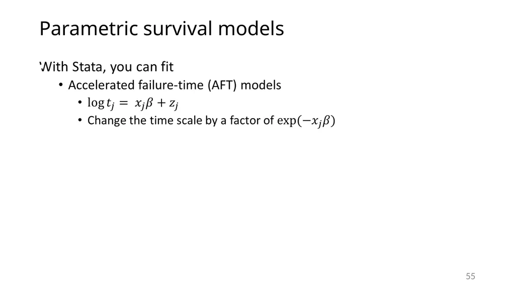
slide55. Parametric survival models 55<br>
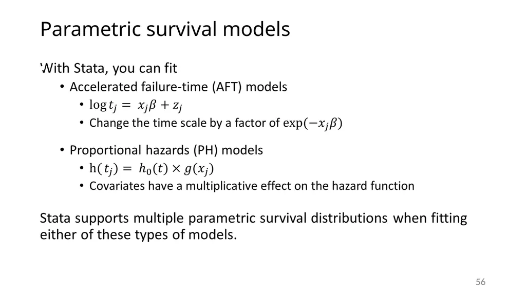
slide56. Parametric survival models 56<br>
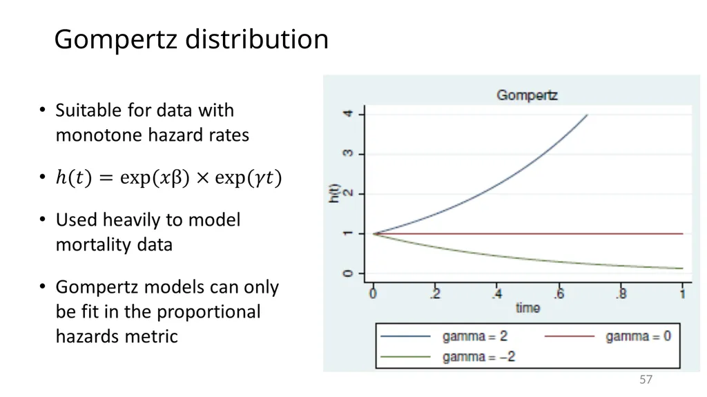
slide57. Gompertz distribution 57<br>
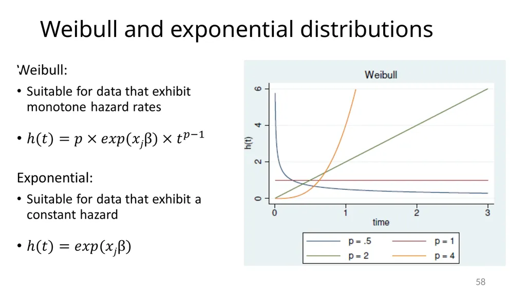
slide58. Weibull and exponential distributions 58<br>
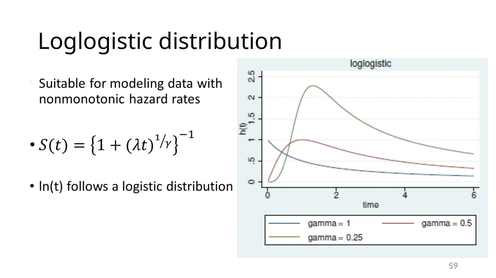
slide59. Loglogistic distribution 59<br>
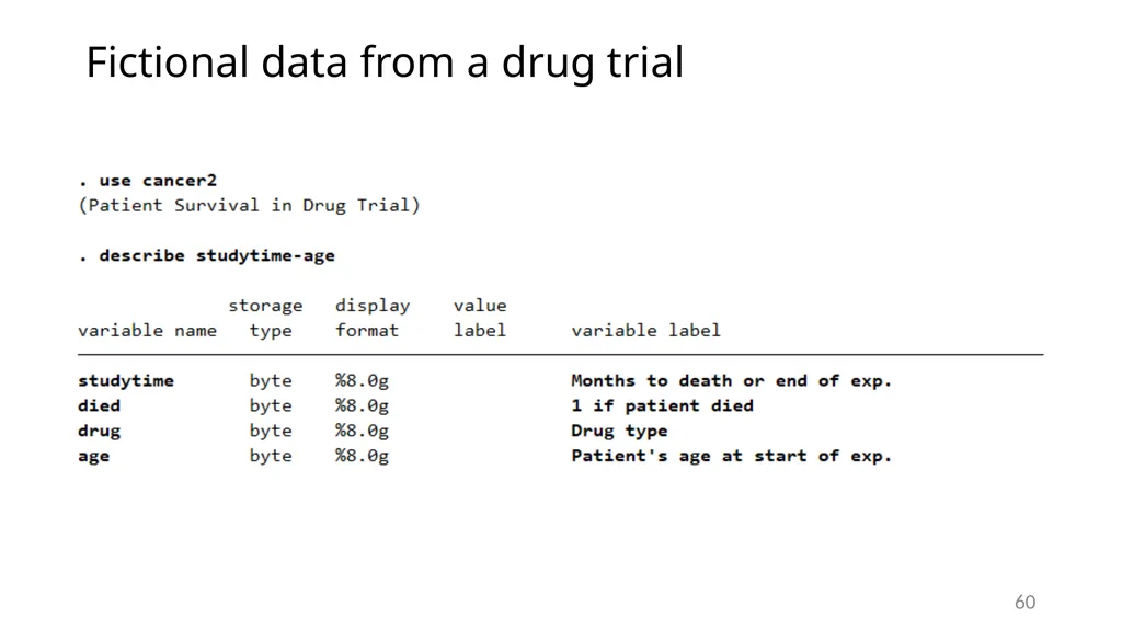
slide60. Fictional data from a drug trial 60<br>
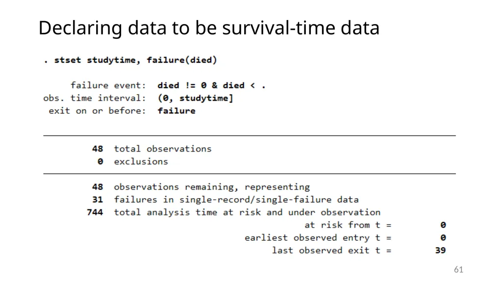
slide61. Declaring data to be survival-time data 61<br>
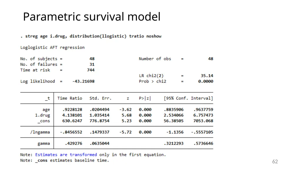
slide62. Parametric survival model 62<br>
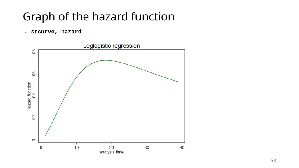
slide63. Graph of the hazard function 63 . stcurve, hazard<br>
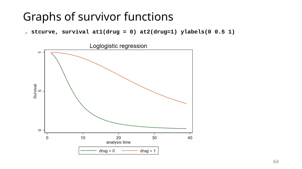
slide64. Graphs of survivor functions 64 . stcurve, survival at1(drug = 0) at2(drug=1) ylabels(0 0.5 1)<br>
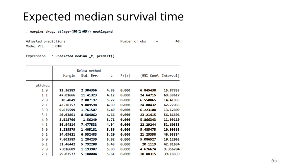
slide65. Expected median survival time 65<br>
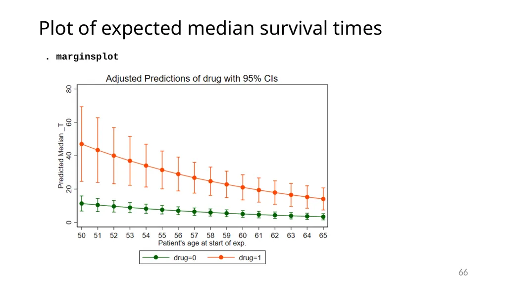
slide66. Plot of expected median survival times 66 . marginsplot<br>
slide67. Interval-censored survival-time data 67<br>
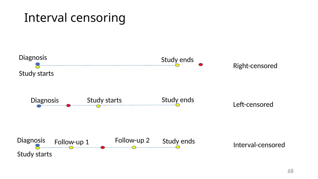
slide68. Interval censoring 68 Diagnosis Study ends Right-censored Diagnosis Study starts Study ends Left-censored Study starts Study starts Study ends Follow-up 1 Follow-up 2 Interval-censored Diagnosis<br>
slide69. Interval-censored survival-time data We fit models for these data with [ST]stintreg
Observations can be uncensored, right-censored, left-censored, or interval-censored
Like [ST]streg, we can fit both AFT and PH models
Unlike with other st commands, data do not need to be stset 69 This Photo by Unknown Author is licensed under CC BY-SA<br>
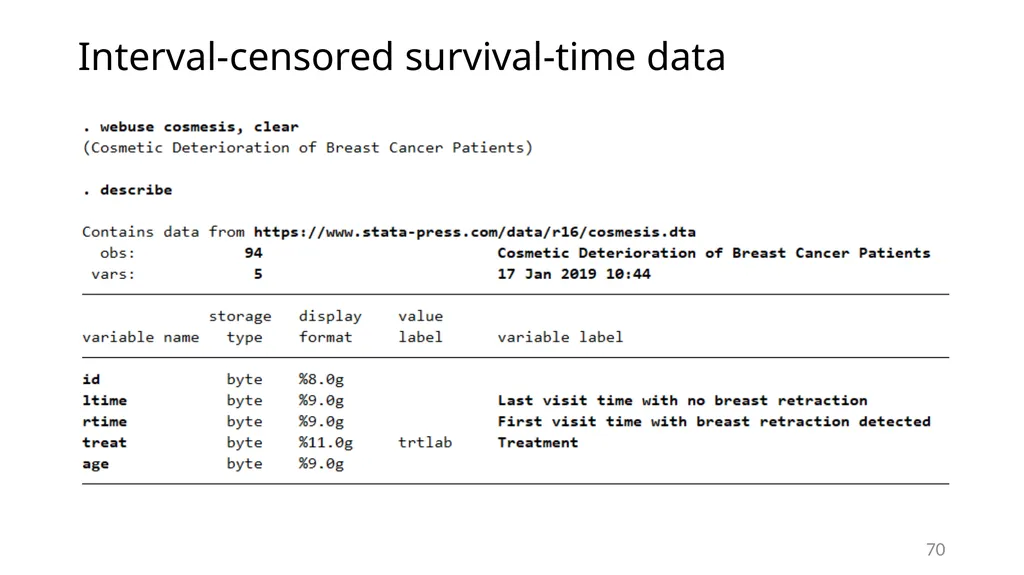
slide70. Interval-censored survival-time data 70<br>
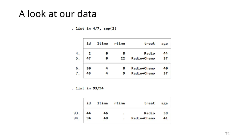
slide71. A look at our data 71<br>
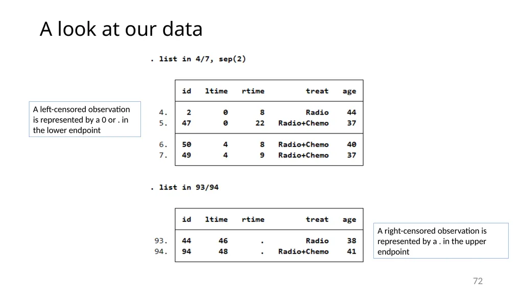
slide72. A look at our data 72 A left-censored observation is represented by a 0 or . in the lower endpoint A right-censored observation is represented by a . in the upper endpoint<br>
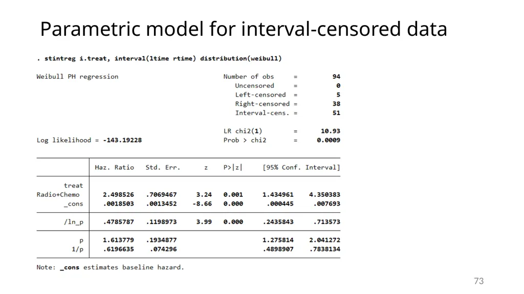
slide73. Parametric model for interval-censored data 73<br>
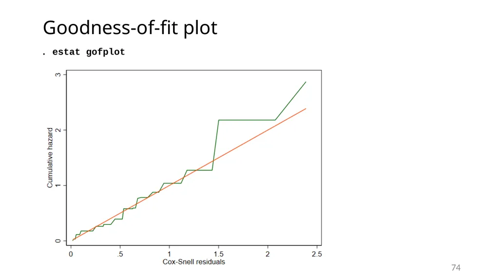
slide74. Goodness-of-fit plot 74 . estat gofplot<br>
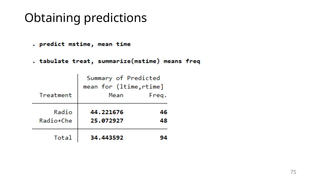
slide75. Obtaining predictions 75<br>
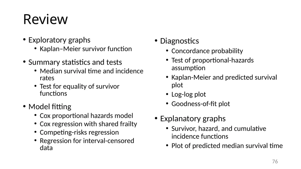
slide76. Review Exploratory graphs
Kaplan–Meier survivor function
Summary statistics and tests
Median survival time and incidence rates
Test for equality of survivor functions
Model fitting
Cox proportional hazards model
Cox regression with shared frailty
Competing-risks regression
Regression for interval-censored data Diagnostics
Concordance probability
Test of proportional-hazards assumption
Kaplan-Meier and predicted survival plot
Log-log plot
Goodness-of-fit plot
Explanatory graphs
Survivor, hazard, and cumulative incidence functions
Plot of predicted median survival time 76<br>
slide77. What else can Stata do with survival data? 77<br>
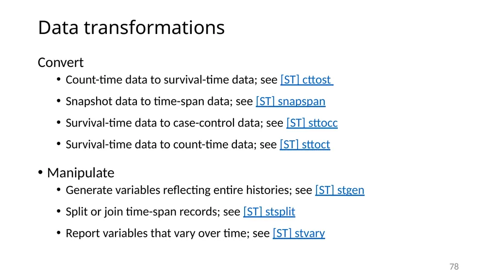
slide78. Data transformations Convert
Count-time data to survival-time data; see [ST] cttost
Snapshot data to time-span data; see [ST] snapspan
Survival-time data to case-control data; see [ST] sttocc
Survival-time data to count-time data; see [ST] sttoct
Manipulate
Generate variables reflecting entire histories; see [ST] stgen
Split or join time-span records; see [ST] stsplit
Report variables that vary over time; see [ST] stvary 78<br>
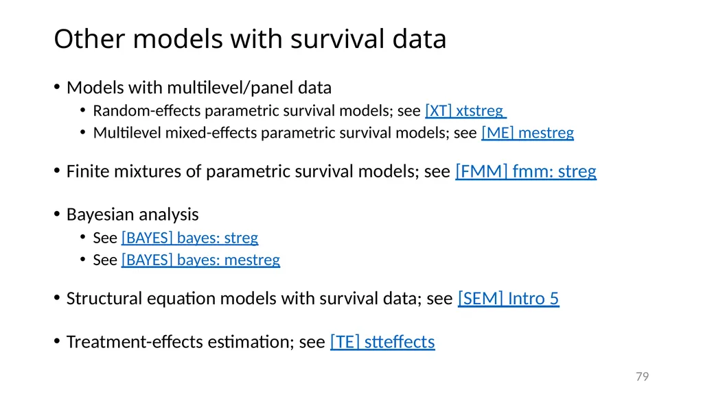
slide79. Other models with survival data Models with multilevel/panel data
Random-effects parametric survival models; see [XT] xtstreg
Multilevel mixed-effects parametric survival models; see [ME] mestreg
Finite mixtures of parametric survival models; see [FMM] fmm: streg
Bayesian analysis
See [BAYES] bayes: streg
See [BAYES] bayes: mestreg
Structural equation models with survival data; see [SEM] Intro 5
Treatment-effects estimation; see [TE] stteffects 79<br>
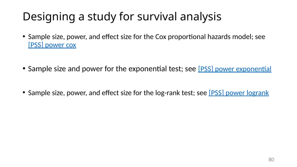
slide80. Designing a study for survival analysis Sample size, power, and effect size for the Cox proportional hazards model; see [PSS] power cox
Sample size and power for the exponential test; see [PSS] power exponential
Sample size, power, and effect size for the log-rank test; see [PSS] power logrank 80<br>
slide81. Where to learn more Overview of Stata’s survival analysis features
Video tutorials on working with survival-time data in Stata
FAQs on working with survival-time models in Stata 81<br>
slide82. References Sun, J. 2006. The Statistical Analysis of Interval-Censored Failure Time Data. New York: Springer
Finkelstein, D. M., and R. A. Wolfe. 1985. A semiparametric model for regression analysis of interval-censored failure time data. Biometrics 41: 933–945.
McGilchrist, C. A., and C. W. Aisbett. 1991. Regression with frailty in survival analysis. Biometrics 47: 461–466. 82<br>

slide83. Thank you 83<br>
slide2. Overview Introduction to survival-time data
Summary statistics
Exploratory graphs
Estimation
Semiparametric and parametric models
Predictions
Diagnostics
Goodness-of-fit plots
Testing assumptions 2<br>
slide3. Introduction to survival data 3<br>
slide4. Survival-time data We measure time to an event of interest
The occurrence of the event is typically called a failure
An observation is censored if we don’t know the exact time of failure
Survival-time data is present in many fields
Health
Economics
Business
Criminology
Stata’s st suite of commands is designed for analyzing survival-time data 4<br>
slide5. A look at survival data 5<br>
slide6. A look at survival data 6 Diagnosis Study ends The patient’s time of death is right-censored if they survive until the end of the study. Died<br>
slide7. Single- vs. multiple-record data 7<br>
slide8. Final notes on survival data There are other varieties
A subject might be diagnosed before the study starts, meaning they are at risk before we observe them (delayed entry).
There might be a gap between the time the subject entered the study and the time the study ended. Suppose the patient was traveling and unable to be reached for a month in the middle of the study but returned before the study ended.
You might have multiple-failure data.
We won’t be focusing on these types of complications, but Stata’s commands for analyzing survival-time data accommodate data with these features. 8<br>
slide9. A first example 9<br>
slide10. A look at survival-time data Before using Stata’s st commands, we need to stset the data. 10<br>
slide11. Declare data to be survival-time data 11<br>
slide12. Describe survival-time data 12<br>
slide13. Kaplan–Meier survivor function 13 . sts graph S(t)=Pr(T>t)<br>
slide14. Kaplan–Meier survivor function by group 14 . sts graph, by(surgery) risktable<br>
slide15. Confidence interval for median survival time 15<br>
slide16. Confidence interval by group 16<br>
slide17. Summary statistics 17<br>
slide18. Other statistics Incidence rates
Obtain estimates and confidence intervals for the incidence-rate ratio (IRR) and incidence-rate difference. See [ST] stir.
Obtain person-time and incidence rate. Also, merge with standard-rate data to obtain SMRs. See [ST] stptime.
Failure rates
Tabulate failure rates by multiple categorical variables
Obtain stratified rate ratios
Carry out trend tests
See [ST] strate.
Life tables
Life, cumulative failure, and hazard tables
Graph survival rate and corresponding confidence interval
See [ST] ltable. 18<br>
slide19. Test equality of survivor functions 19<br>
slide20. Cox proportional hazards model 20<br>
slide21. Single-observation survival-time data 21<br>
slide22. Display survival-time settings 22<br>
slide23. Survivor and hazard functions 23 . sts graph, surv saving(survival)
. sts graph, hazard nob saving(hazard)
. graph combine survival hazard<br>
slide24. Cox proportional hazards model 24<br>
slide25. Cox proportional hazards model 25<br>
slide26. Survivor function 26 . stcurve, survival<br>
slide27. Survivor function 27 . stcurve, survival
at1(drug=0 age=50)
at2(drug=0 age=60)
at3(drug=1 age=50)
at4(drug=1 age=60)<br>
slide28. Hazard function 28 . stcurve, hazard
at1(drug=0) at2(drug=1)<br>
slide29. Assessing our model Statistics
How well do our predictions agree with the outcomes?
Does the proportional-hazards assumption hold?
Diagnostic plots
Plot of residuals versus time
Log-log plots
Comparison of the observed survival curve and the Cox predicted curve 29<br>
slide30. Concordance probability 30<br>
slide31. Test the proportional hazards assumption 31<br>
slide32. Plotting Schoenfeld residuals versus time 32 . estat phtest, plot(drug)<br>
slide33. . stphplot, by(drug) Log-log plot 33<br>
slide34. . stcoxkm, by(drug) Kaplan–Meier and predicted survival plots 34<br>
slide35. More on the proportional-hazards assumption Graphical assessment of the proportional-hazards assumption
Log-log plots
Adjust the estimates to average values of specified variables
Kaplan–Meier and predicted survival plots
Specify the method to handle tied failures
Test the proportional-hazards assumption
Test using Schoenfeld residuals
Choose from other time-scale functions or specify your own function of time
To learn more, see [ST]stcox PH-assumption tests. 35<br>
slide36. Interaction between a covariate and analysis time 36<br>
slide37. Shared-frailty models 37<br>
slide38. Shared-frailty models 38<br>
slide39. Shared-frailty data 39<br>
slide40. Declare data to be survival-time data 40<br>
slide41. Cox regression with shared frailty 41<br>
slide42. Estimates of log frailties 42<br>
slide43. Estimates of log frailties 43<br>
slide44. Other variations of the Cox model Stratified Cox regression
Group specific baseline hazard
. stcox x1 x2, strata(svar)
Select another method to handle tied failures
Efron, exact marginal-likelihood, or exact partial-likelihood
Learn more about fitting a Cox proportional hazards model in [ST]stcox. 44<br>
slide45. Competing risks regression models 45<br>
slide46. Competing failure events Consider patients in an ICU after having a heart attack
Model the time until a cardiac arrest
If a patient dies, they are no longer at risk for cardiac arrest
The event of death competes with our event of interest
With this type of data, we want to focus on the cumulative incidence function 46<br>
slide47. Cumulative incidence function 47 CIF(t)=Pr(T≤t and event of interest)<br>
slide48. Hazards for competing risks 48<br>
slide49. Subhazard 49<br>
slide50. Data with competing failure events 50<br>
slide51. Declare data to be survival-time data 51<br>
slide52. Competing risks regression 52<br>
slide53. Graph of cumulative incidence function 53 . stcurve, cif at1(pneumonia=0) at2(pneumonia=1)<br>
slide54. Parametric survival models 54<br>
slide55. Parametric survival models 55<br>
slide56. Parametric survival models 56<br>
slide57. Gompertz distribution 57<br>
slide58. Weibull and exponential distributions 58<br>
slide59. Loglogistic distribution 59<br>
slide60. Fictional data from a drug trial 60<br>
slide61. Declaring data to be survival-time data 61<br>
slide62. Parametric survival model 62<br>
slide63. Graph of the hazard function 63 . stcurve, hazard<br>
slide64. Graphs of survivor functions 64 . stcurve, survival at1(drug = 0) at2(drug=1) ylabels(0 0.5 1)<br>
slide65. Expected median survival time 65<br>
slide66. Plot of expected median survival times 66 . marginsplot<br>
slide67. Interval-censored survival-time data 67<br>
slide68. Interval censoring 68 Diagnosis Study ends Right-censored Diagnosis Study starts Study ends Left-censored Study starts Study starts Study ends Follow-up 1 Follow-up 2 Interval-censored Diagnosis<br>
slide69. Interval-censored survival-time data We fit models for these data with [ST]stintreg
Observations can be uncensored, right-censored, left-censored, or interval-censored
Like [ST]streg, we can fit both AFT and PH models
Unlike with other st commands, data do not need to be stset 69 This Photo by Unknown Author is licensed under CC BY-SA<br>
slide70. Interval-censored survival-time data 70<br>
slide71. A look at our data 71<br>
slide72. A look at our data 72 A left-censored observation is represented by a 0 or . in the lower endpoint A right-censored observation is represented by a . in the upper endpoint<br>
slide73. Parametric model for interval-censored data 73<br>
slide74. Goodness-of-fit plot 74 . estat gofplot<br>
slide75. Obtaining predictions 75<br>
slide76. Review Exploratory graphs
Kaplan–Meier survivor function
Summary statistics and tests
Median survival time and incidence rates
Test for equality of survivor functions
Model fitting
Cox proportional hazards model
Cox regression with shared frailty
Competing-risks regression
Regression for interval-censored data Diagnostics
Concordance probability
Test of proportional-hazards assumption
Kaplan-Meier and predicted survival plot
Log-log plot
Goodness-of-fit plot
Explanatory graphs
Survivor, hazard, and cumulative incidence functions
Plot of predicted median survival time 76<br>
slide77. What else can Stata do with survival data? 77<br>
slide78. Data transformations Convert
Count-time data to survival-time data; see [ST] cttost
Snapshot data to time-span data; see [ST] snapspan
Survival-time data to case-control data; see [ST] sttocc
Survival-time data to count-time data; see [ST] sttoct
Manipulate
Generate variables reflecting entire histories; see [ST] stgen
Split or join time-span records; see [ST] stsplit
Report variables that vary over time; see [ST] stvary 78<br>
slide79. Other models with survival data Models with multilevel/panel data
Random-effects parametric survival models; see [XT] xtstreg
Multilevel mixed-effects parametric survival models; see [ME] mestreg
Finite mixtures of parametric survival models; see [FMM] fmm: streg
Bayesian analysis
See [BAYES] bayes: streg
See [BAYES] bayes: mestreg
Structural equation models with survival data; see [SEM] Intro 5
Treatment-effects estimation; see [TE] stteffects 79<br>
slide80. Designing a study for survival analysis Sample size, power, and effect size for the Cox proportional hazards model; see [PSS] power cox
Sample size and power for the exponential test; see [PSS] power exponential
Sample size, power, and effect size for the log-rank test; see [PSS] power logrank 80<br>
slide81. Where to learn more Overview of Stata’s survival analysis features
Video tutorials on working with survival-time data in Stata
FAQs on working with survival-time models in Stata 81<br>
slide82. References Sun, J. 2006. The Statistical Analysis of Interval-Censored Failure Time Data. New York: Springer
Finkelstein, D. M., and R. A. Wolfe. 1985. A semiparametric model for regression analysis of interval-censored failure time data. Biometrics 41: 933–945.
McGilchrist, C. A., and C. W. Aisbett. 1991. Regression with frailty in survival analysis. Biometrics 47: 461–466. 82<br>
slide83. Thank you 83<br>