
Treewidth and Fix Parameter Tractability. Bounded
KB
Published · 62 slides · 0 views
1 / 1

Description
Treewidth and Fix Parameter Tractability. Bounded treewidth is interesting Even more so in the context of Fixed Parameter tractability. How close is a graph to being a tree? It has constant treewidth if every subgraph has a constant size
Related Topics
Share
Embed code
Download this presentation From Below
"Treewidth and Fix Parameter Tractability. Bounded" is the property of its rightful owner. Permission is granted to download and print the materials on this website for personal, non-commercial use only, and to display it on your personal computer provided you do not modify the materials and that you retain all copyright notices contained in the materials. By downloading content from our website, you accept the terms of this agreement.
Presentation Transcript
01
Treewidth and Fix Parameter Tractability. Bounded treewidth is interesting
Even more so in the context of Fixed Parameter tractability.
How close is a graph to being a tree?
It has constant treewidth if every subgraph has a constant size separator.<br>
Even more so in the context of Fixed Parameter tractability.
How close is a graph to being a tree?
It has constant treewidth if every subgraph has a constant size separator.<br>
02
Examples Series Parallel graphs. These are exactly the graphs with treewidth 2. Look for definition in the web.
An outerplanar graph, namely a graph that can be
mapped to the plane so that all the vertices are in the outer phase, has tree width 2. Cactus graphs, Pseudoforeest, Halin graphs, Apollonian graphs,
chordal graphs with a maximum clique bounded by a
constant, and Planar graphs with diameter k have treewidth at most 3k.<br>
03
I will use Chandra Chekuri’s notes on treewidth but modified. Studied by [Halin’76]
Again by [Robertson & Seymour’84] as part of their seminal graph minor project<br>
Again by [Robertson & Seymour’84] as part of their seminal graph minor project<br>
04
Treewidth Informal: treewidth(G) k implies G can be recursively decomposed via “balanced” separators of size k
(A measure tailored for a given graph)
Formal: see next slide.<br>
(A measure tailored for a given graph)
Formal: see next slide.<br>
05
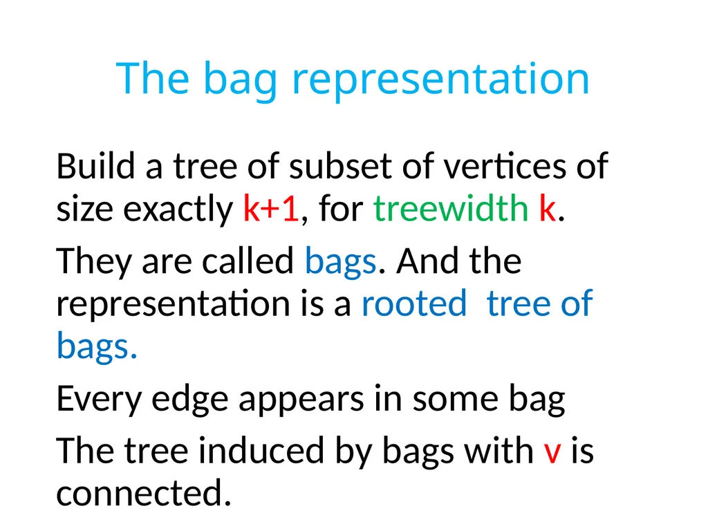
The bag representation Build a tree of subset of vertices of size exactly k+1, for treewidth k.
They are called bags. And the representation is a rooted tree of bags.
Every edge appears in some bag
The tree induced by bags with v is connected.<br>
They are called bags. And the representation is a rooted tree of bags.
Every edge appears in some bag
The tree induced by bags with v is connected.<br>
06
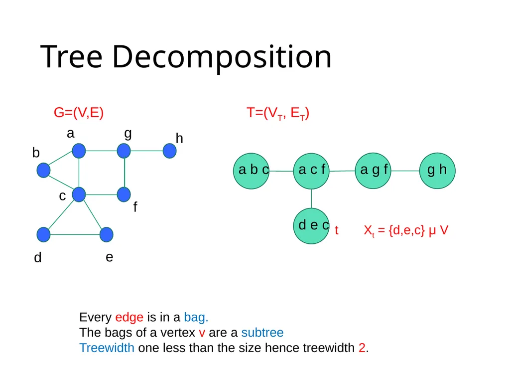
Tree Decomposition a b c a c f d e c a g f g h G=(V,E) T=(VT, ET) t Xt = {d,e,c} µ V Every edge is in a bag.
The bags of a vertex v are a subtree
Treewidth one less than the size hence treewidth 2.<br>
The bags of a vertex v are a subtree
Treewidth one less than the size hence treewidth 2.<br>
07
This means something strong Say that I have a leaf bag. I decide that v is in the solution. This means that I have a tree for which all the bags contain v.
Thus I do not have to deal with v anymore.
Thus it is additive not multiplicative. We do not have to guess for v in any other bag.<br>
Thus I do not have to deal with v anymore.
Thus it is additive not multiplicative. We do not have to guess for v in any other bag.<br>
08
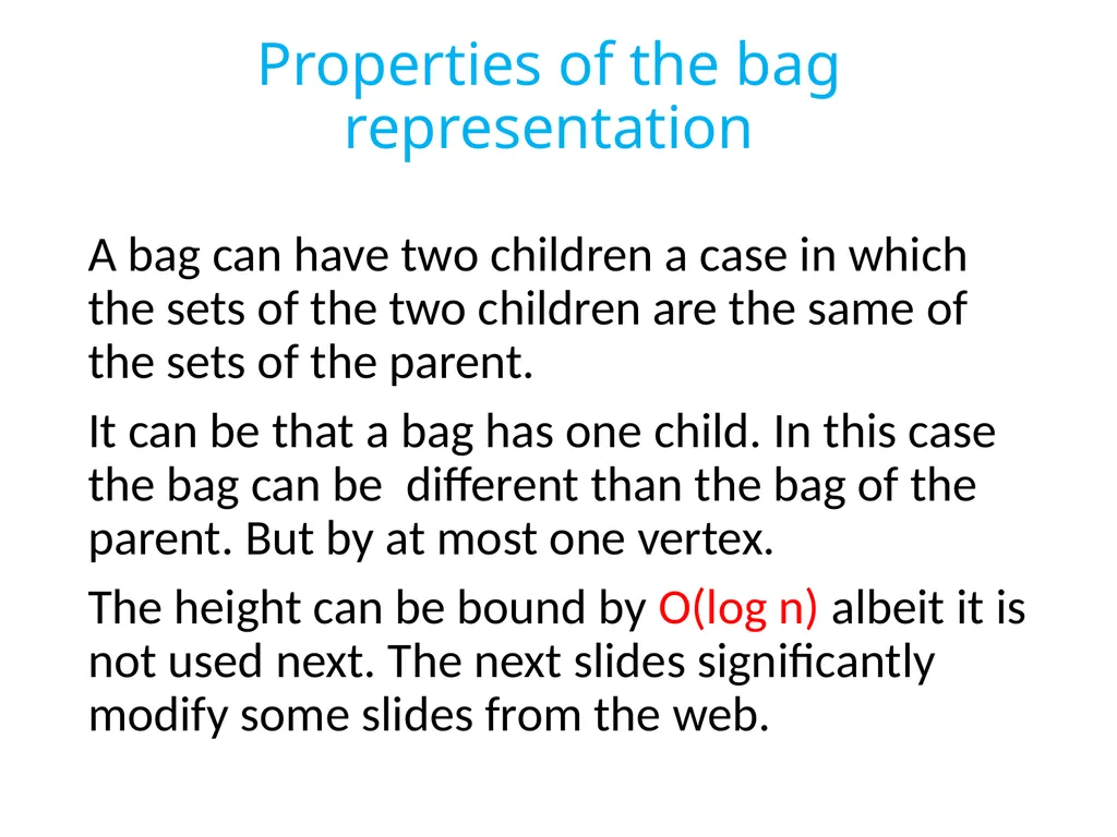
Properties of the bag representation A bag can have two children a case in which the sets of the two children are the same of the sets of the parent.
It can be that a bag has one child. In this case the bag can be different than the bag of the parent. But by at most one vertex.
The height can be bound by O(log n) albeit it is not used next. The next slides significantly modify some slides from the web.<br>
It can be that a bag has one child. In this case the bag can be different than the bag of the parent. But by at most one vertex.
The height can be bound by O(log n) albeit it is not used next. The next slides significantly modify some slides from the web.<br>
09
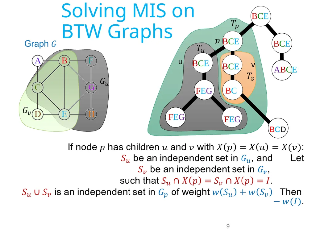
Solving MIS on
BTW Graphs 9 Feg BC bce abce bce bce Feg Feg bce bce u v BCD<br>
10
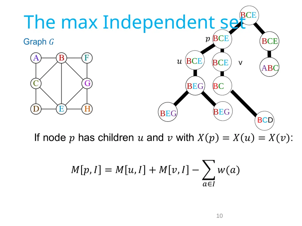
10 bce beg bcE BC bce abc bce The max Independent set beg beg bce v BCD<br>
11
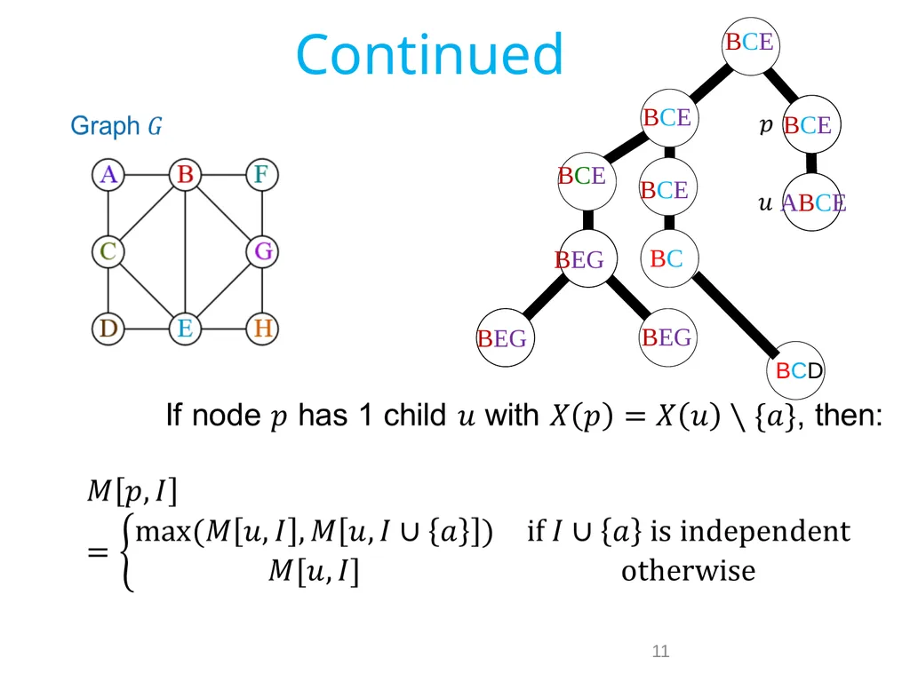
11 bce beg Bc bce abcE bce bce Continued beg beg bCE BCD<br>
12
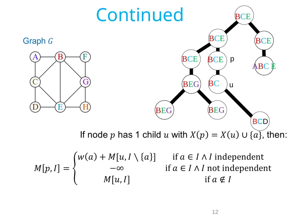
12 bce beg Bc bce Abc e bce bce Continued bCe beg beg p u BCD<br>
13
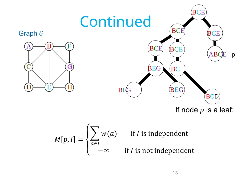
13 bce beg BC bfg bce AbcE bce bce Continued bce beg p BCD<br>
14
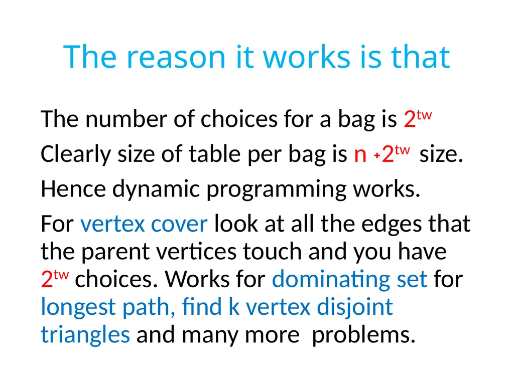
The reason it works is that The number of choices for a bag is 2tw
Clearly size of table per bag is n ˖2tw size.
Hence dynamic programming works.
For vertex cover look at all the edges that the parent vertices touch and you have 2tw choices. Works for dominating set for longest path, find k vertex disjoint triangles and many more problems.<br>
Clearly size of table per bag is n ˖2tw size.
Hence dynamic programming works.
For vertex cover look at all the edges that the parent vertices touch and you have 2tw choices. Works for dominating set for longest path, find k vertex disjoint triangles and many more problems.<br>
15
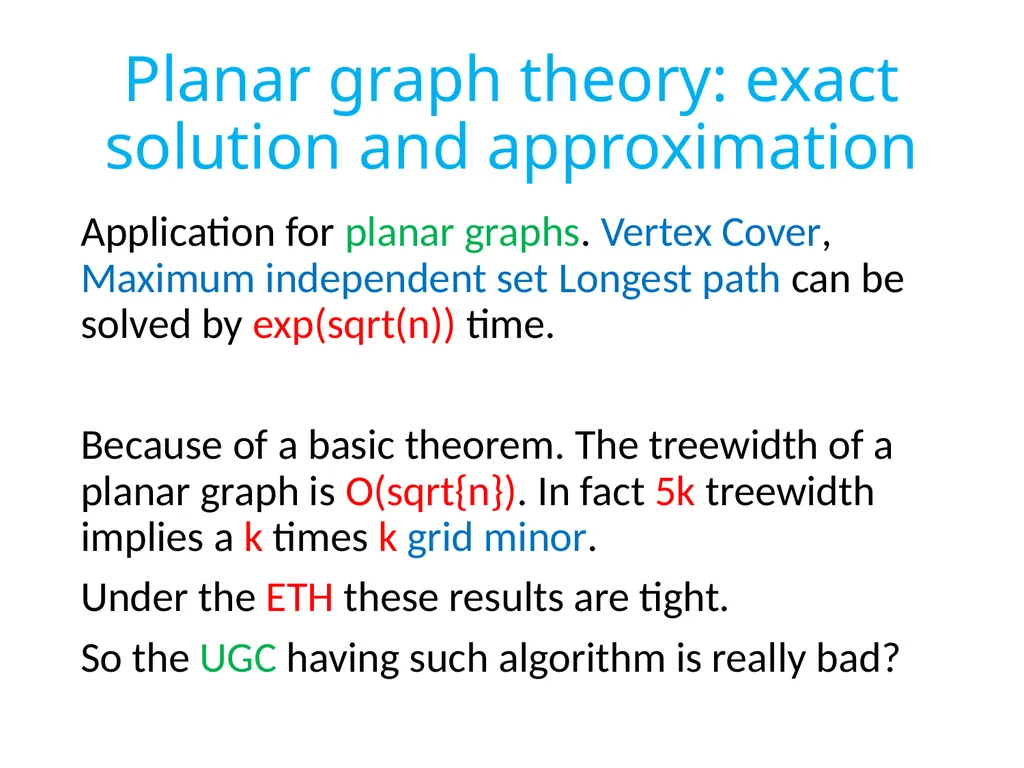
Planar graph theory: exact solution and approximation Application for planar graphs. Vertex Cover, Maximum independent set Longest path can be solved by exp(sqrt(n)) time.
Because of a basic theorem. The treewidth of a planar graph is O(sqrt{n}). In fact 5k treewidth implies a k times k grid minor.
Under the ETH these results are tight.
So the UGC having such algorithm is really bad?<br>
Because of a basic theorem. The treewidth of a planar graph is O(sqrt{n}). In fact 5k treewidth implies a k times k grid minor.
Under the ETH these results are tight.
So the UGC having such algorithm is really bad?<br>
16
The Baker method I use (modified) slides of Chekuri.
Defining the number of faces L. Remove the outer face in the graph, and recourse. The number of faces we find is called L. Enumerate the faces from 1 to L.
We may assume that given any constant ε>0
L> 1/ε4 (otherwise there is an exact solution). Take d such that L/d= 1/ε2 , (assume for simplicity all numbers are integers).
Define h graphs, for h=1/ε2 V1, ..., Vh<br>
17
The graphs Vj for j≤h are all faces with indices
j, j+h,j+2h, j+3h….. And remove them.
The graph Vj is a union of disjoint outerplanar graphs. This is not needed for
Maximum (cost) Independent Set. But it is essential in many coloring problems I worked on.
What remains are disjoint graphs of diameter h-1.<br>
j, j+h,j+2h, j+3h….. And remove them.
The graph Vj is a union of disjoint outerplanar graphs. This is not needed for
Maximum (cost) Independent Set. But it is essential in many coloring problems I worked on.
What remains are disjoint graphs of diameter h-1.<br>
18
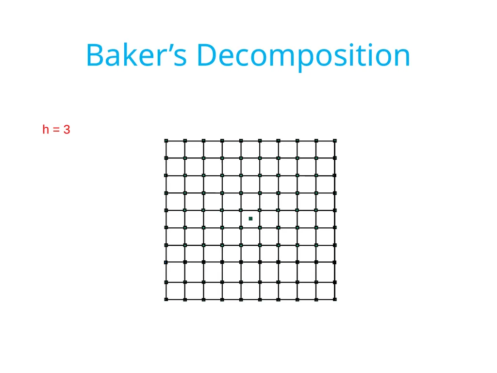
Baker’s Decomposition h = 3<br>
19
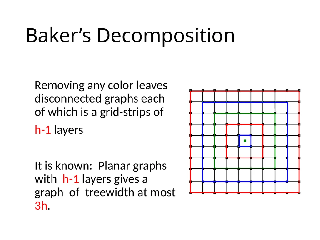
Baker’s Decomposition Removing any color leaves disconnected graphs each of which is a grid-strips of
h-1 layers
It is known: Planar graphs with h-1 layers gives a graph of treewidth at most 3h.<br>
h-1 layers
It is known: Planar graphs with h-1 layers gives a graph of treewidth at most 3h.<br>
20
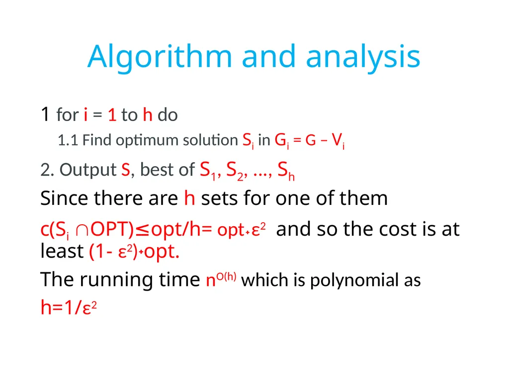
Algorithm and analysis 1 for i = 1 to h do
1.1 Find optimum solution Si in Gi = G – Vi
2. Output S, best of S1, S2, ..., Sh
Since there are h sets for one of them
c(Si OPT)≤opt/h= opt˖ε2 and so the cost is at least (1- ε2)˖opt.
The running time nO(h) which is polynomial as
h=1/ε2<br>
1.1 Find optimum solution Si in Gi = G – Vi
2. Output S, best of S1, S2, ..., Sh
Since there are h sets for one of them
c(Si OPT)≤opt/h= opt˖ε2 and so the cost is at least (1- ε2)˖opt.
The running time nO(h) which is polynomial as
h=1/ε2<br>
21
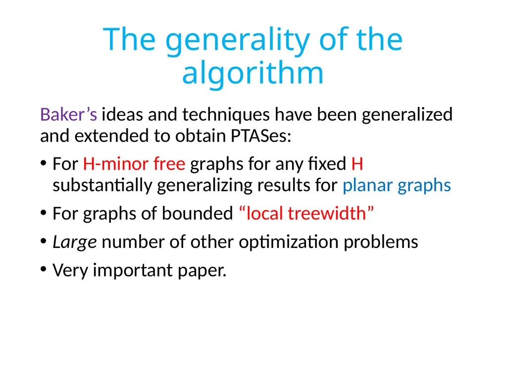
The generality of the algorithm Baker’s ideas and techniques have been generalized and extended to obtain PTASes:
For H-minor free graphs for any fixed H substantially generalizing results for planar graphs
For graphs of bounded “local treewidth”
Large number of other optimization problems
Very important paper.<br>
For H-minor free graphs for any fixed H substantially generalizing results for planar graphs
For graphs of bounded “local treewidth”
Large number of other optimization problems
Very important paper.<br>
22
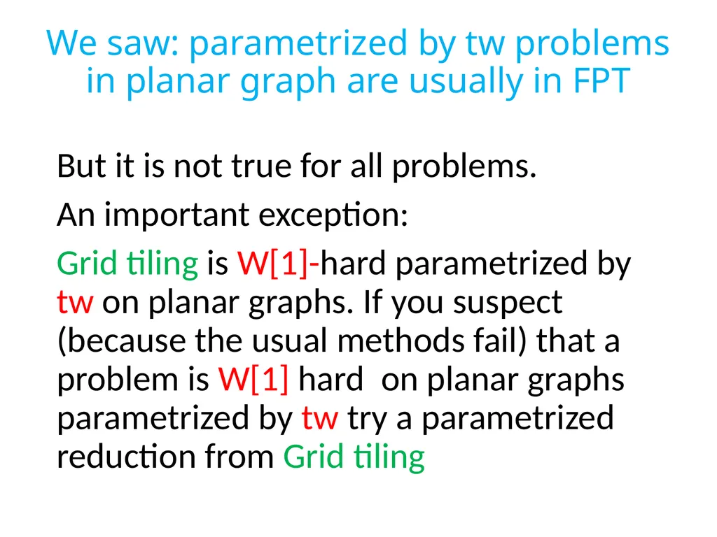
We saw: parametrized by tw problems in planar graph are usually in FPT But it is not true for all problems.
An important exception:
Grid tiling is W[1]-hard parametrized by tw on planar graphs. If you suspect (because the usual methods fail) that a problem is W[1] hard on planar graphs parametrized by tw try a parametrized reduction from Grid tiling<br>
An important exception:
Grid tiling is W[1]-hard parametrized by tw on planar graphs. If you suspect (because the usual methods fail) that a problem is W[1] hard on planar graphs parametrized by tw try a parametrized reduction from Grid tiling<br>
23
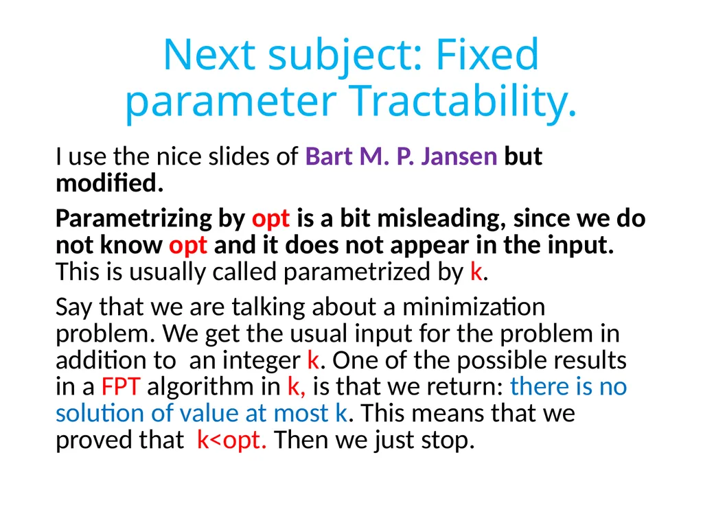
Next subject: Fixed parameter Tractability. I use the nice slides of Bart M. P. Jansen but modified.
Parametrizing by opt is a bit misleading, since we do not know opt and it does not appear in the input. This is usually called parametrized by k.
Say that we are talking about a minimization problem. We get the usual input for the problem in addition to an integer k. One of the possible results in a FPT algorithm in k, is that we return: there is no solution of value at most k. This means that we proved that k<opt. Then we just stop.<br>
24
Continued The second possibility is that we output a solution of size k. Since we can not know opt, it may be that k>opt maybe by a lot. But this also happens when you binary search for the value of opt.
Since we return a solution of size k, clearly k≥opt. Since we allow time f(k) for any computable function f we are also are allowed time f(opt) for any f.
Hence parametrized algorithm by k may fail to return an answer and say k<opt. Next we see two example in which k is not the parameter.<br>
Since we return a solution of size k, clearly k≥opt. Since we allow time f(k) for any computable function f we are also are allowed time f(opt) for any f.
Hence parametrized algorithm by k may fail to return an answer and say k<opt. Next we see two example in which k is not the parameter.<br>
25
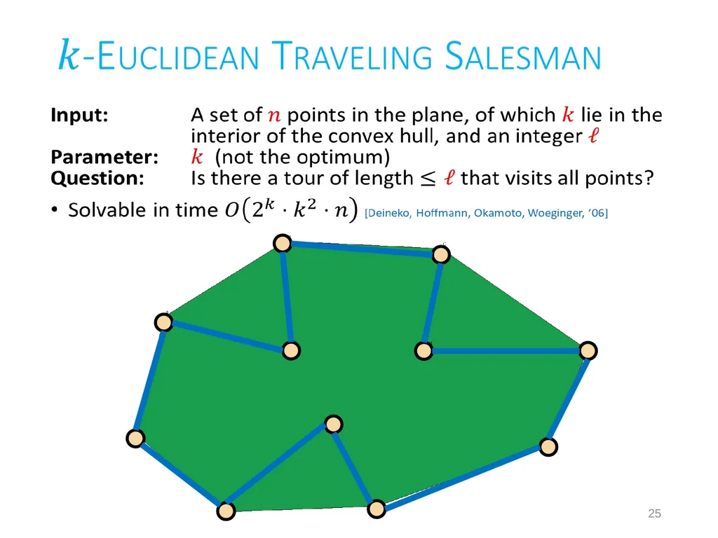
25<br>
26
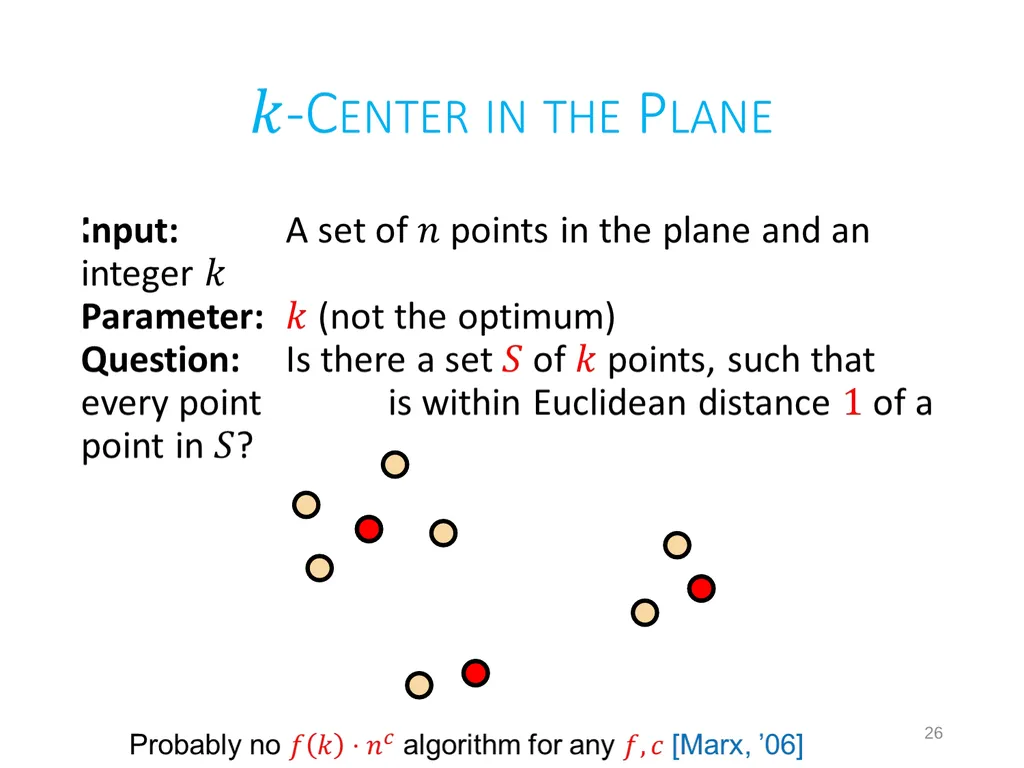
26<br>
27
Can a set of points in the plane be covered by k lines? No reason to take a line that covers one point.
Hence the number of candidates lines is k2
The algorithm:
1) As long as there is a line that covers k points take it.
2) If there are more than k2 points left as every line covers at most k-1 points return k<opt.
3) Else apply some exponential algorithm on the k2
points<br>
Hence the number of candidates lines is k2
The algorithm:
1) As long as there is a line that covers k points take it.
2) If there are more than k2 points left as every line covers at most k-1 points return k<opt.
3) Else apply some exponential algorithm on the k2
points<br>
28
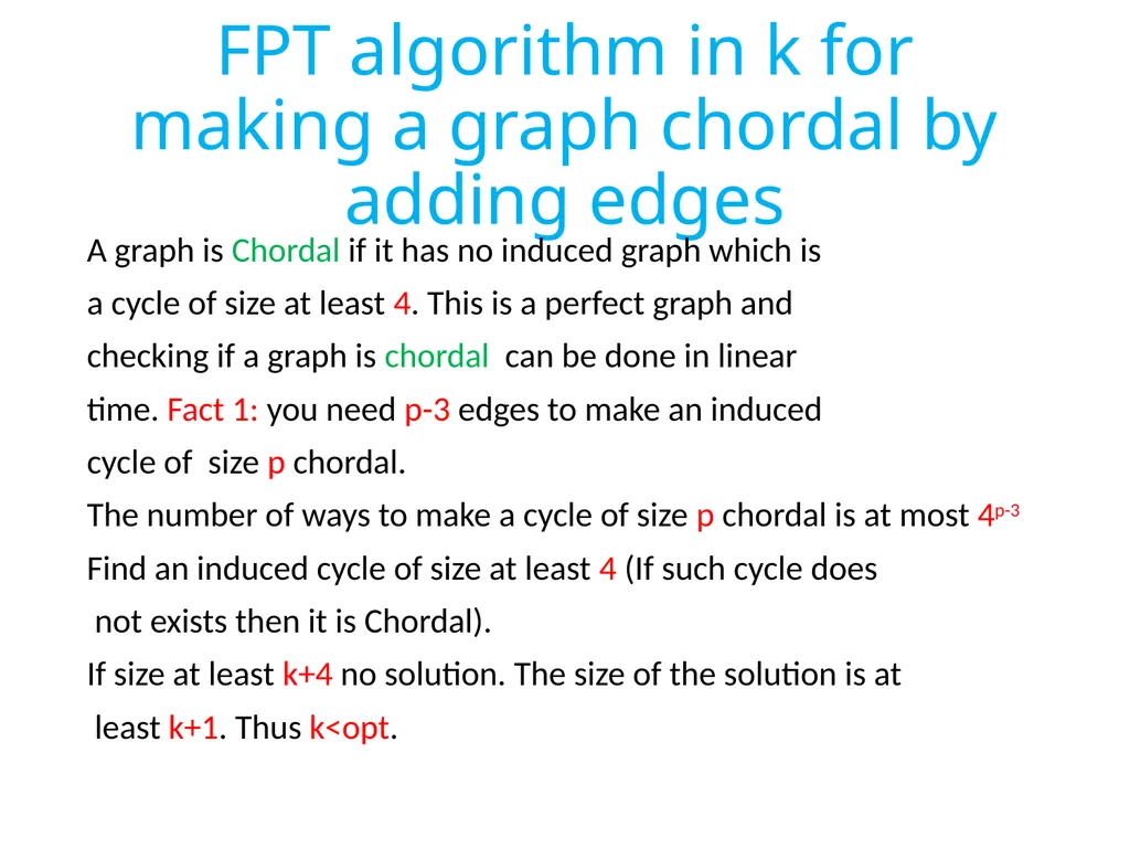
FPT algorithm in k for making a graph chordal by adding edges A graph is Chordal if it has no induced graph which is
a cycle of size at least 4. This is a perfect graph and
checking if a graph is chordal can be done in linear
time. Fact 1: you need p-3 edges to make an induced
cycle of size p chordal.
The number of ways to make a cycle of size p chordal is at most 4p-3
Find an induced cycle of size at least 4 (If such cycle does
not exists then it is Chordal).
If size at least k+4 no solution. The size of the solution is at
least k+1. Thus k<opt.<br>
29
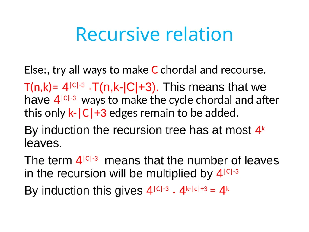
Recursive relation Else:, try all ways to make C chordal and recourse.
T(n,k)= 4|C|-3 ˖T(n,k-|C|+3). This means that we have 4|C|-3 ways to make the cycle chordal and after this only k-|C|+3 edges remain to be added.
By induction the recursion tree has at most 4k leaves.
The term 4|C|-3 means that the number of leaves in the recursion will be multiplied by 4|C|-3
By induction this gives 4|C|-3 ˖ 4k-|c|+3 = 4k<br>
30
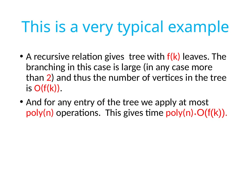
This is a very typical example A recursive relation gives tree with f(k) leaves. The branching in this case is large (in any case more than 2) and thus the number of vertices in the tree is O(f(k)).
And for any entry of the tree we apply at most poly(n) operations. This gives time poly(n)˖O(f(k)).<br>
And for any entry of the tree we apply at most poly(n) operations. This gives time poly(n)˖O(f(k)).<br>
31
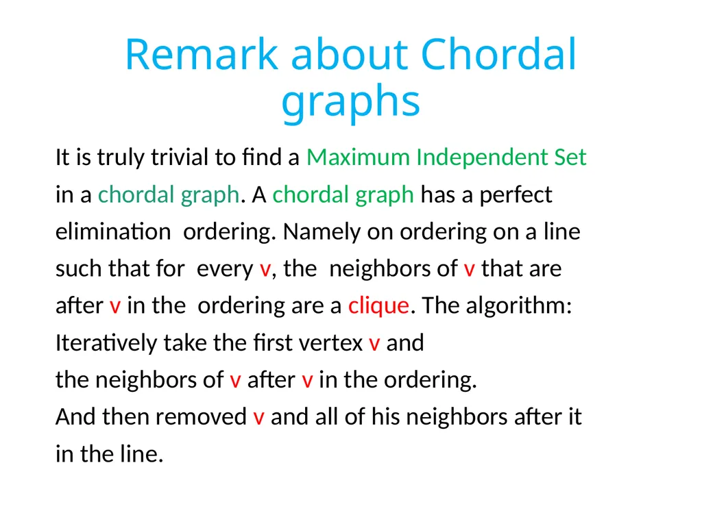
Remark about Chordal graphs It is truly trivial to find a Maximum Independent Set
in a chordal graph. A chordal graph has a perfect
elimination ordering. Namely on ordering on a line
such that for every v, the neighbors of v that are
after v in the ordering are a clique. The algorithm:
Iteratively take the first vertex v and
the neighbors of v after v in the ordering.
And then removed v and all of his neighbors after it
in the line.<br>
32
Continued This gives a decomposition of the graph to cliques.
Say that there are k cliques. Since after we remove v
we also remove all its neighbors, each clique gives
one vertex to an independent set. Thus the
independent set has size k, and because the graph
was decomposed into k cliques, this independent set
is maximum.<br>
Say that there are k cliques. Since after we remove v
we also remove all its neighbors, each clique gives
one vertex to an independent set. Thus the
independent set has size k, and because the graph
was decomposed into k cliques, this independent set
is maximum.<br>
33
Continued This also solves the problem: decompose G to
minimum number of cliques, namely the problem of
minimum coloring of the complement graph of G.
This is not surprising. The complement of a perfect graph is perfect as well hence has a polynomial time algorithm for minimum coloring.<br>
minimum number of cliques, namely the problem of
minimum coloring of the complement graph of G.
This is not surprising. The complement of a perfect graph is perfect as well hence has a polynomial time algorithm for minimum coloring.<br>
34
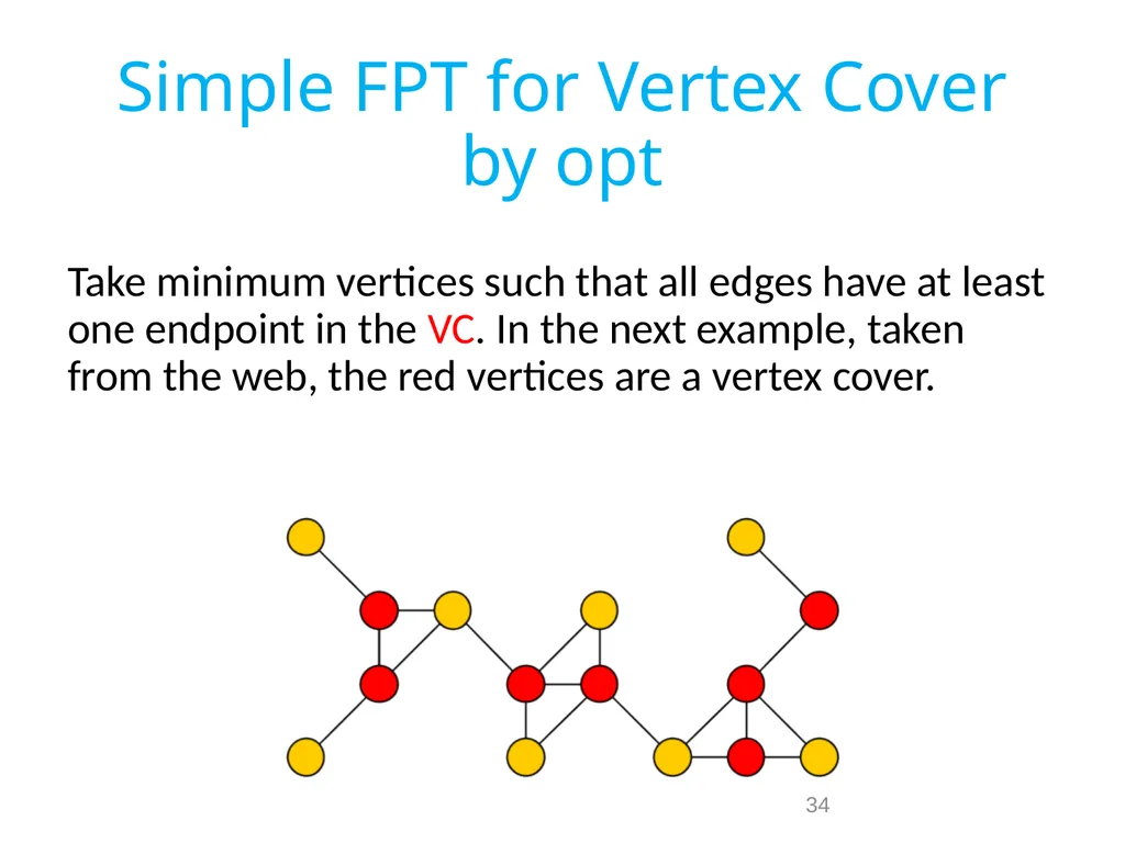
Simple FPT for Vertex Cover by opt Take minimum vertices such that all edges have at least one endpoint in the VC. In the next example, taken from the web, the red vertices are a vertex cover. 34<br>
35
The decision tree Edge decision binary tree. Parameter k.
Each choice for uv: Either u is in or v is in.
Every path in every direction chooses a vertex. Therefore every path must stop at length k. Indeed if a solution is not found for this height, it means that k<opt.<br>
Each choice for uv: Either u is in or v is in.
Every path in every direction chooses a vertex. Therefore every path must stop at length k. Indeed if a solution is not found for this height, it means that k<opt.<br>
36
This is called a kernel We reduced the problem to a tree of size 2k.
Means that VC can be solved in time 2k poly(n). This is called fixed parameter tractable in the in k.
I sometime call it FPT in the optimum.
Finding a kernel is equivalent to FPT.<br>
Means that VC can be solved in time 2k poly(n). This is called fixed parameter tractable in the in k.
I sometime call it FPT in the optimum.
Finding a kernel is equivalent to FPT.<br>
37
Similar for covering triangles A tree diverges acceding to which vertex of the 3 is taken to the solution.
In any path we choose k after the path gets to length k.
Hence the kernel has size 3k<br>
In any path we choose k after the path gets to length k.
Hence the kernel has size 3k<br>
38
FPT in k for shortest path Color the vertices by random k colors. Say that there is a path of length k. A path is colorful if all colors are different. Probability k!/ kk which is around 1/ ek. Doing it ek ˖ n times gives probability of exp(-n) of failure. This can be derandomized by universal hash functions.
Finding a colorful path if exists requires
2k poly(n) time by DP. This method is called Color Coding.<br>
Finding a colorful path if exists requires
2k poly(n) time by DP. This method is called Color Coding.<br>
39
Hamiltonian Cycle Hamiltonian cycle has kernel of size kk
You just combine partial paths.
In 2013 that the problem was given 4k Kernel size.
Not a simple matter since HC is much more global.
I think this paper is clever.<br>
You just combine partial paths.
In 2013 that the problem was given 4k Kernel size.
Not a simple matter since HC is much more global.
I think this paper is clever.<br>
40
Sketch First give weights at random and make the
solution unique (The Isolation lemma I knew it
from derandomization and from RNC algorithm
or Perfect Matching)
Consider all min cost cycle cover and color each cycle
by black or red.
Count the number of different colorings of optimum solutions. If there is a
Hamiltonian path it adds 2 to the number of colorings.
Every cover by several cycles will have at least 4 colorings.<br>
41
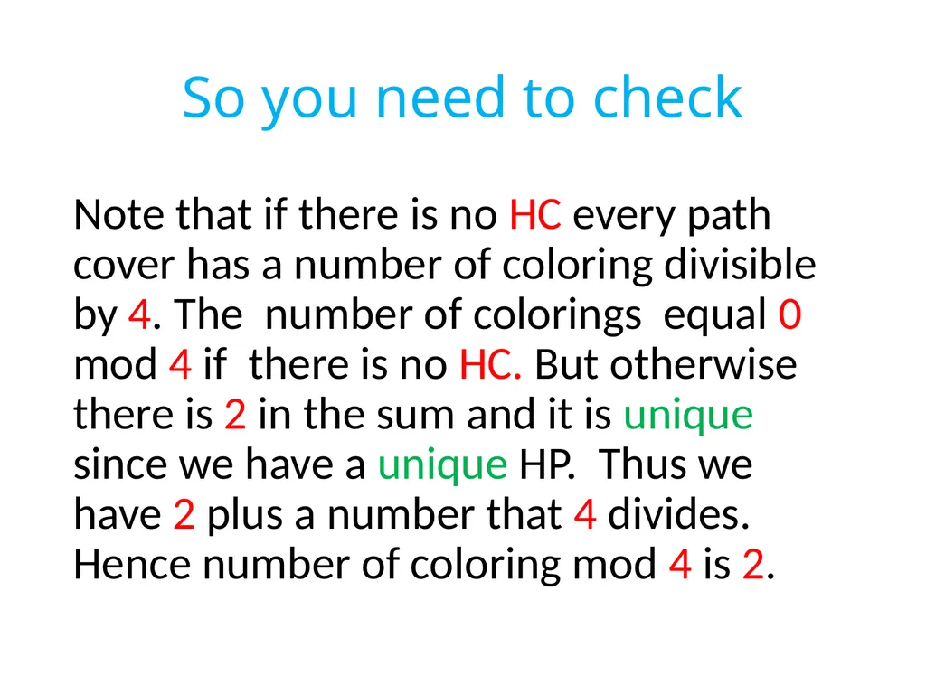
So you need to check Note that if there is no HC every path cover has a number of coloring divisible by 4. The number of colorings equal 0 mod 4 if there is no HC. But otherwise there is 2 in the sum and it is unique since we have a unique HP. Thus we have 2 plus a number that 4 divides. Hence number of coloring mod 4 is 2.<br>
42
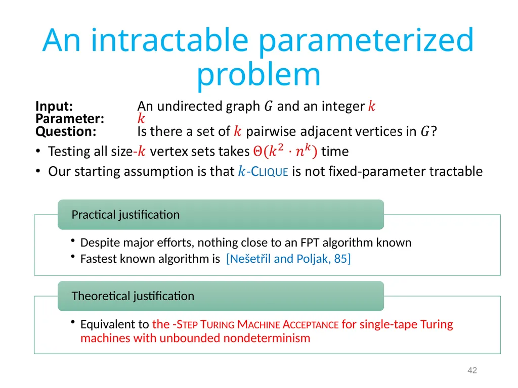
An intractable parameterized problem 42<br>
43
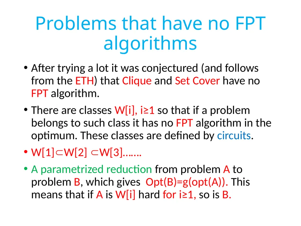
Problems that have no FPT algorithms After trying a lot it was conjectured (and follows from the ETH) that Clique and Set Cover have no FPT algorithm.
There are classes W[i], i≥1 so that if a problem belongs to such class it has no FPT algorithm in the optimum. These classes are defined by circuits.
W[1]W[2] W[3]…….
A parametrized reduction from problem A to problem B, which gives Opt(B)=g(opt(A)). This means that if A is W[i] hard for i≥1, so is B.<br>
44
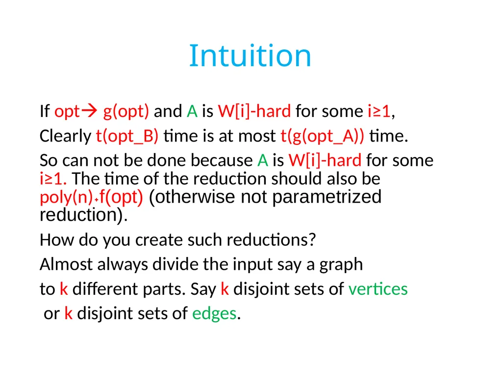
Intuition If opt g(opt) and A is W[i]-hard for some i≥1,
Clearly t(opt_B) time is at most t(g(opt_A)) time.
So can not be done because A is W[i]-hard for some i≥1. The time of the reduction should also be poly(n)˖f(opt) (otherwise not parametrized reduction).
How do you create such reductions?
Almost always divide the input say a graph
to k different parts. Say k disjoint sets of vertices
or k disjoint sets of edges.<br>
45
Set-Cover and Clique. Clique is in W[1] while Set-Cover is in W[2].
There is a parametrized reduction from Clique to Set-Cover but not vise-versa. In that very weak sense
Set-Cover is the harder.
It is known that Clique has no o(opt) ratio in time
t(opt)poly(n) for any function t.
For Set –Cover there is no r(opt) approximation that runs in time t(opt)poly(n) for an r and t. These are called Total Fixed Parameter Inapproximability.<br>
46
Combining approximation and FPT If the problem is W[i]-hard for some i≥1 and it
either has a very bad approximation or some
threshold that was not broken for a long time, we
should allow time f(k) for some parameter k and any f.
Combine FPT and approximation to get a better result.
Consider the k-cut problem. Remove minimum cost
collection of edges so that the graph G will
decomposed to at least k components.
A paper of Gupta et al gave a 2-ε ratio for some
constant ε if the problem is parametrized by k.<br>
47
A very good reason to allow parametrization in approximation Recall that Manurangsi gave a lower bound of 2 for the
k-cut problem under the Small Set Expansion
Conjecture. Hence if you want to break the 2 you have
to relax the problem. As another example consider the
Minimum Cost Strongly Connected Subgraph problem. This
problem is W[1]-hard and has a terrible nε approximation
ratio which we do not expect to improve (the ratio comes
from the algorithm for the Directed Steiner Tree problem).
But if you parametrized by k you get ratio 2. See a paper by
Chitins et al in the references.<br>
48
An example: allowing FPT time gives a PTAS We discuss the following problem. Given a graph and
a number k, find a set U of k vertices and maximize
the number of edges touching U. Under the SSEC this problem admits no better than ratio 2.
Ratio 2 is trivial. To improve the ratio we parametrize the problem by k (which in this case is definitely not the optimum).
First step: Make opt bounded by a function of k.
Let D=C(k,2)/ε (C(k,2) is k choose 2).<br>
49
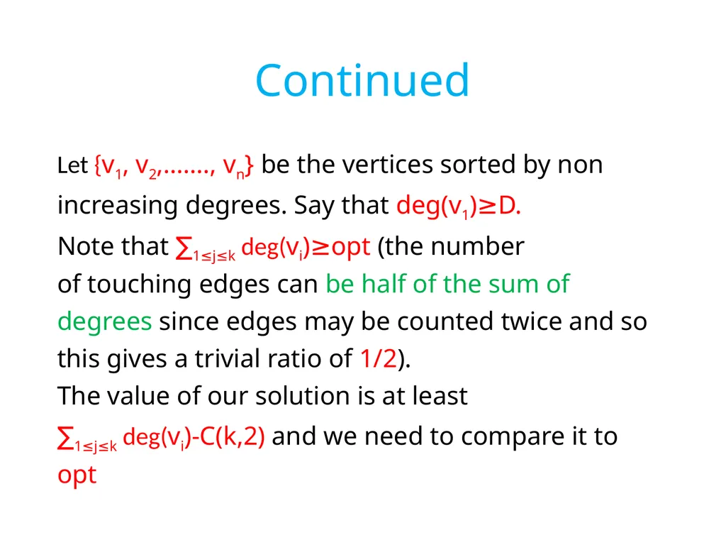
Continued Let {v1, v2,……., vn} be the vertices sorted by non
increasing degrees. Say that deg(v1)≥D.
Note that ∑1≤j≤k deg(vi)≥opt (the number
of touching edges can be half of the sum of
degrees since edges may be counted twice and so
this gives a trivial ratio of 1/2).
The value of our solution is at least
∑1≤j≤k deg(vi)-C(k,2) and we need to compare it to
opt<br>
50
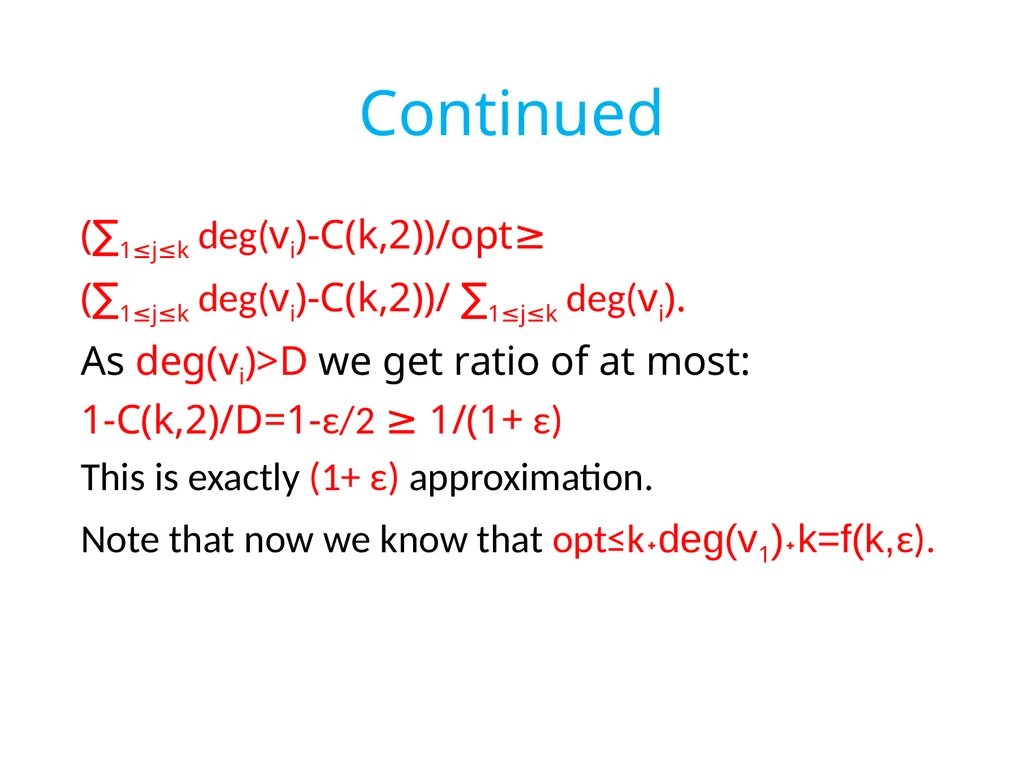
Continued (∑1≤j≤k deg(vi)-C(k,2))/opt≥
(∑1≤j≤k deg(vi)-C(k,2))/ ∑1≤j≤k deg(vi).
As deg(vi)>D we get ratio of at most:
1-C(k,2)/D=1-ε/2 ≥ 1/(1+ ε)
This is exactly (1+ ε) approximation.
Note that now we know that opt≤k˖deg(v1)˖k=f(k,ε).<br>
(∑1≤j≤k deg(vi)-C(k,2))/ ∑1≤j≤k deg(vi).
As deg(vi)>D we get ratio of at most:
1-C(k,2)/D=1-ε/2 ≥ 1/(1+ ε)
This is exactly (1+ ε) approximation.
Note that now we know that opt≤k˖deg(v1)˖k=f(k,ε).<br>
51
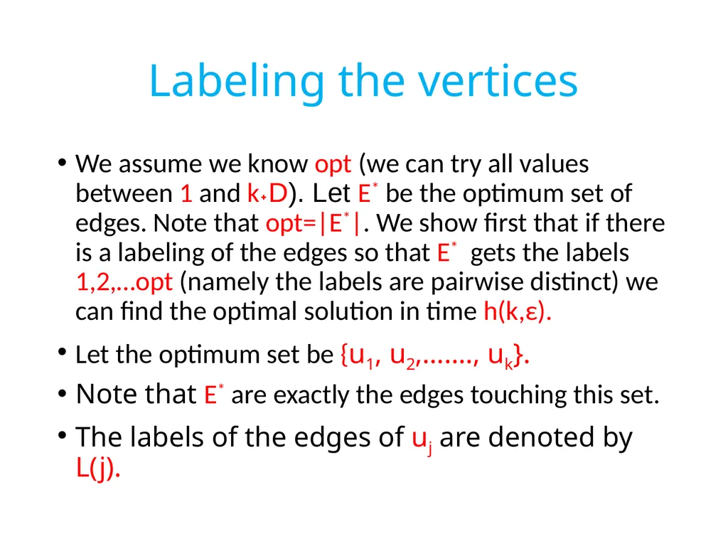
Labeling the vertices We assume we know opt (we can try all values between 1 and k˖D). Let E* be the optimum set of edges. Note that opt=|E*|. We show first that if there is a labeling of the edges so that E* gets the labels 1,2,…opt (namely the labels are pairwise distinct) we can find the optimal solution in time h(k,ε).
Let the optimum set be {u1, u2,……., uk}.
Note that E* are exactly the edges touching this set.
The labels of the edges of uj are denoted by L(j).<br>
Let the optimum set be {u1, u2,……., uk}.
Note that E* are exactly the edges touching this set.
The labels of the edges of uj are denoted by L(j).<br>
52
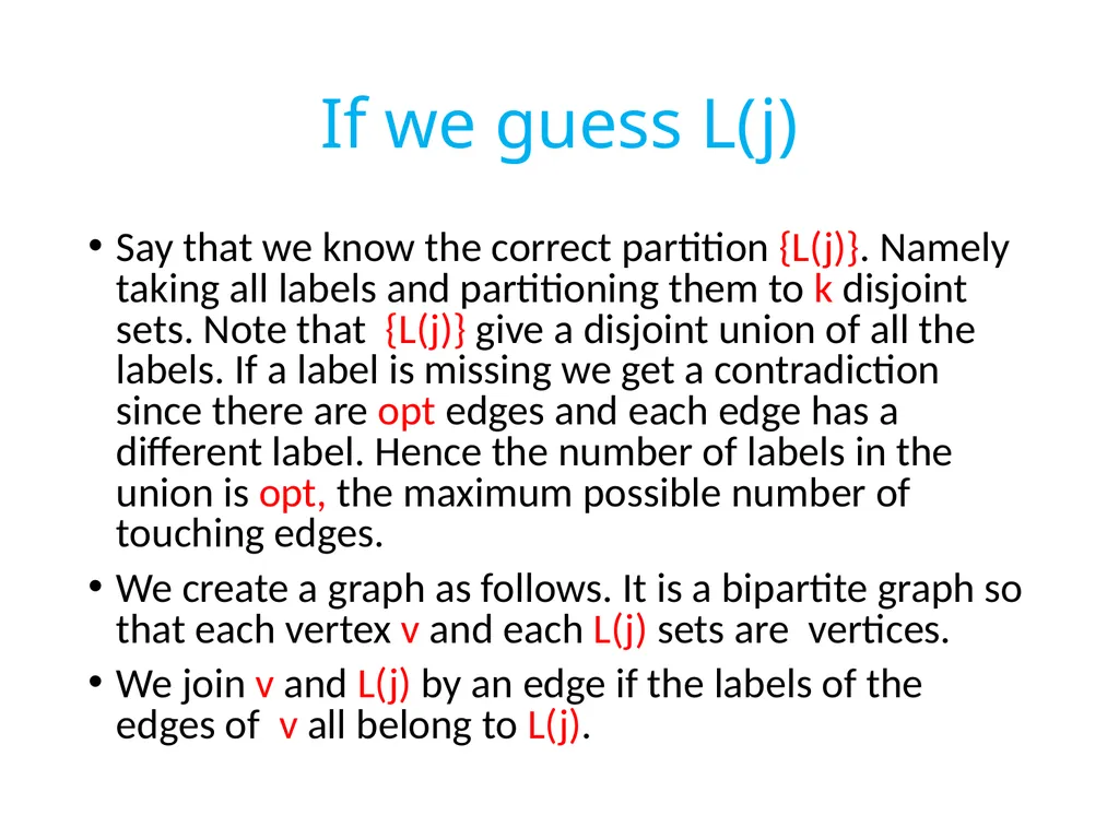
If we guess L(j) Say that we know the correct partition {L(j)}. Namely taking all labels and partitioning them to k disjoint sets. Note that {L(j)} give a disjoint union of all the labels. If a label is missing we get a contradiction since there are opt edges and each edge has a different label. Hence the number of labels in the union is opt, the maximum possible number of touching edges.
We create a graph as follows. It is a bipartite graph so that each vertex v and each L(j) sets are vertices.
We join v and L(j) by an edge if the labels of the edges of v all belong to L(j).<br>
We create a graph as follows. It is a bipartite graph so that each vertex v and each L(j) sets are vertices.
We join v and L(j) by an edge if the labels of the edges of v all belong to L(j).<br>
53
If we have a matching containing all L(j) sets This means that we found k vertices with opt labels and since the labels are pairwise disjoint,
the vertices are touched by opt edges. Namely we
found the optimum solution. The number of partitions is kopt To get the correct partition it is enough to make the random experiment n˖
kopt times and with probability 1-exp(-n) one of the partitions will be the correct one.
Color Coding again.<br>
the vertices are touched by opt edges. Namely we
found the optimum solution. The number of partitions is kopt To get the correct partition it is enough to make the random experiment n˖
kopt times and with probability 1-exp(-n) one of the partitions will be the correct one.
Color Coding again.<br>
54
Continued To start it all, we need the labels of E* to be
different. The probability for that is 1/optopt
And so doing it say n˖optopt times guarantees with probability at least 1-exp(-n) one of the trials will give the edges of E* different labels. Again Color Coding.
This PTAS is an adaptation of a PTAS of Marx for another problem. Hence the result I just described is due to Daniel Marx.<br>
55
Parameter that is not opt continued Say that we are given a graph that is not planar,
and a set X={v1, v2,……., vk} of vertices whose
removal creates a Planar Graph. What is the best
approximation for coloring if we parametrized by k?
We can guess the coloring of X in time kk .
The rest of the vertices can be colored by 4 colors.
Let the number of colors of X be opt.
The optimum may get a coloring by only opt.
The ratio is (opt+4)/opt.<br>
56
The ratio If X is 1 colorable or 2 colorable we can check. The worst case is that X is 4 colorable. And we get a ratio of (opt+4)/opt=2. Without parametrizing by k we can not get anything.
Definition: an EPTAS is a 1+ε approximation that runs in time f(ε).Poly(n).
Claim: if a problem is W[j] hard for j ≥1, it does not admits an EPTAS approximation.
This is one of the only relations between FPT and approximation that I know.<br>
Definition: an EPTAS is a 1+ε approximation that runs in time f(ε).Poly(n).
Claim: if a problem is W[j] hard for j ≥1, it does not admits an EPTAS approximation.
This is one of the only relations between FPT and approximation that I know.<br>
57
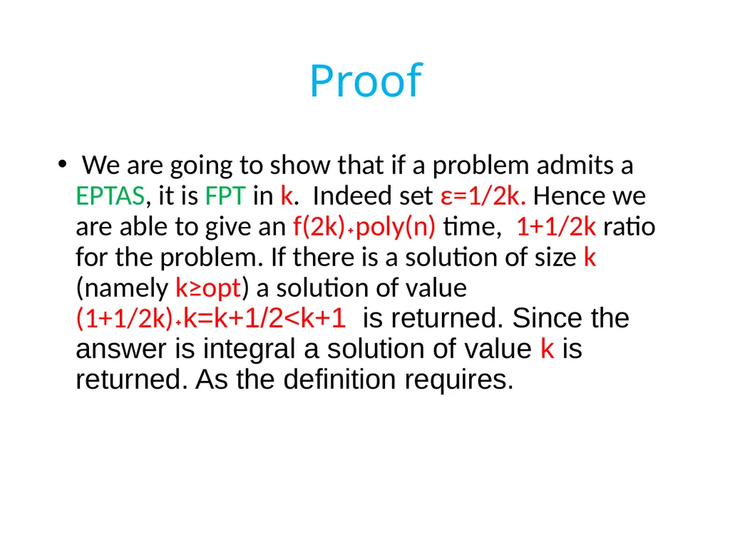
Proof We are going to show that if a problem admits a EPTAS, it is FPT in k. Indeed set ε=1/2k. Hence we are able to give an f(2k)˖poly(n) time, 1+1/2k ratio for the problem. If there is a solution of size k (namely k≥opt) a solution of value (1+1/2k)˖k=k+1/2<k+1 is returned. Since the answer is integral a solution of value k is returned. As the definition requires.<br>
58
Continued If the optimum is at least k+1 the solution returns
a solution of value (1+1/2k)(k+1)≥k+1.
This is evidence that k<opt.
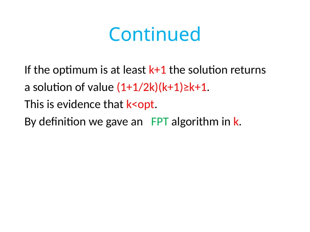
By definition we gave an FPT algorithm in k.<br>
a solution of value (1+1/2k)(k+1)≥k+1.
This is evidence that k<opt.
By definition we gave an FPT algorithm in k.<br>
59
Favorite open problem What is the best approximation for Set-Cover in terms of the sets?
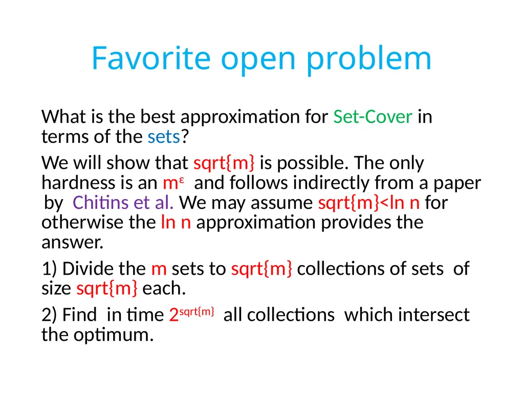
We will show that sqrt{m} is possible. The only hardness is an mε and follows indirectly from a paper by Chitins et al. We may assume sqrt{m}<ln n for otherwise the ln n approximation provides the answer.
1) Divide the m sets to sqrt{m} collections of sets of size sqrt{m} each.
2) Find in time 2sqrt{m} all collections which intersect the optimum.<br>
60
Continued 3) For every collection which intersects the
optimum, add ALL the sets of the collection into the
solution.
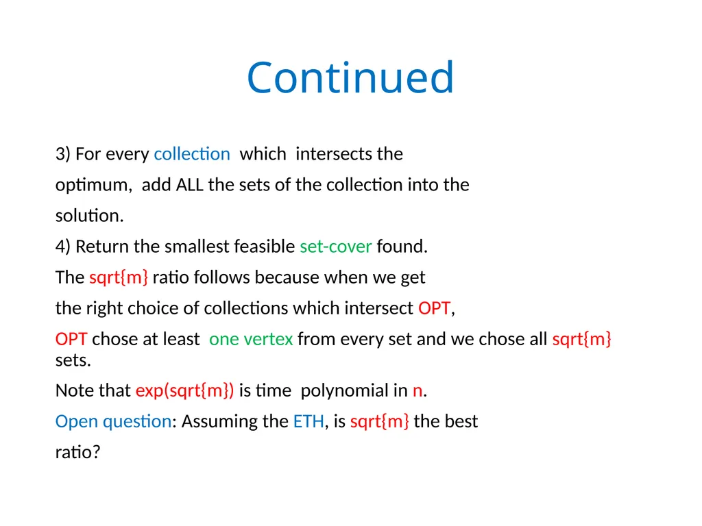
4) Return the smallest feasible set-cover found.
The sqrt{m} ratio follows because when we get
the right choice of collections which intersect OPT,
OPT chose at least one vertex from every set and we chose all sqrt{m} sets.
Note that exp(sqrt{m}) is time polynomial in n.
Open question: Assuming the ETH, is sqrt{m} the best
ratio?<br>
61
Is there some real relation between FPT and approximation? It does not seem so to me at all.
Set-Cover which is W[2]-hard has better approximation than Clique which belongs to W[1].
Problems with very bad ratio like Directed Steiner tree are FPT in k.
Bad approximation does not mean anything in the
FPT world. And being W[i] hard for some i≥1,
does not mean the ratio is bad.<br>
Set-Cover which is W[2]-hard has better approximation than Clique which belongs to W[1].
Problems with very bad ratio like Directed Steiner tree are FPT in k.
Bad approximation does not mean anything in the
FPT world. And being W[i] hard for some i≥1,
does not mean the ratio is bad.<br>
62
Fix parameter inapproximability is a young subject However, there are several surveys on FPT
approximation. And they have some
inapproximability results. Until recently the PCP was
not used in fixed parameter inapproximability (not
sure why). Then almost linear PCP were suggested and used.
A wide open question: give Total Fixed Parameter
Inapproximability for coloring.
A wide open question: give good fix parameter
inapproximability for the Dense k-Subgraph problem.<br>