
UDM Msc course in education & development 2013
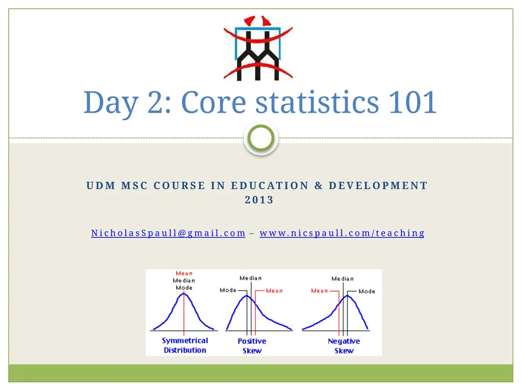
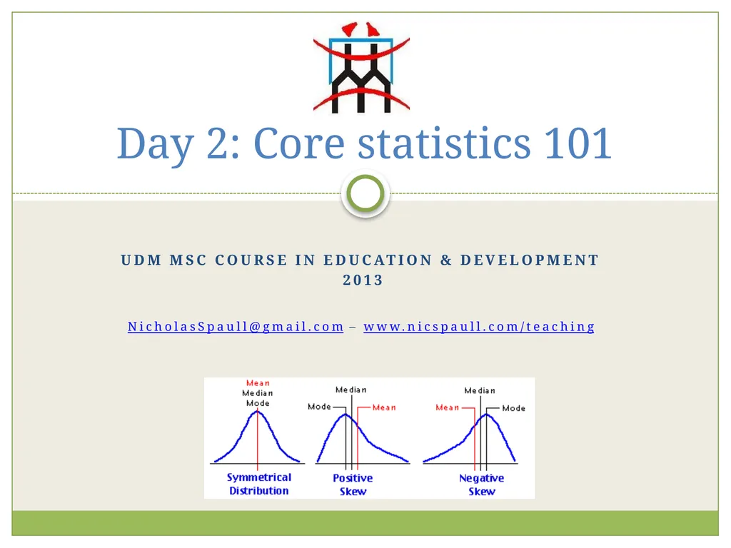

Description: UDM Msc course in education development 2013 NicholasSpaullgmail.com www.nicspaull.comteaching Day 2: Core statistics 101 Introduction What are statistics? the practice or science of collecting and analysing numerical data in large
Related Topics
Download Presentation
"UDM Msc course in education & development 2013" is the property of its rightful owner. Permission is granted to download and print the materials on this website for personal, non-commercial use only, and to display it on your personal computer provided you do not modify the materials and that you retain all copyright notices contained in the materials. By downloading content from our website, you accept the terms of this agreement.
Presentation Transcript
slide1. UDM Msc course in education & development
2013
NicholasSpaull@gmail.com – www.nicspaull.com/teaching Day 2: Core statistics 101<br>
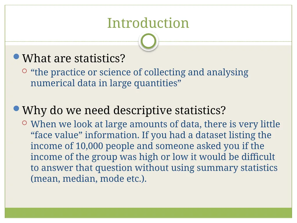
slide2. Introduction What are statistics?
“the practice or science of collecting and analysing numerical data in large quantities”
Why do we need descriptive statistics?
When we look at large amounts of data, there is very little “face value” information. If you had a dataset listing the income of 10,000 people and someone asked you if the income of the group was high or low it would be difficult to answer that question without using summary statistics (mean, median, mode etc.).<br>
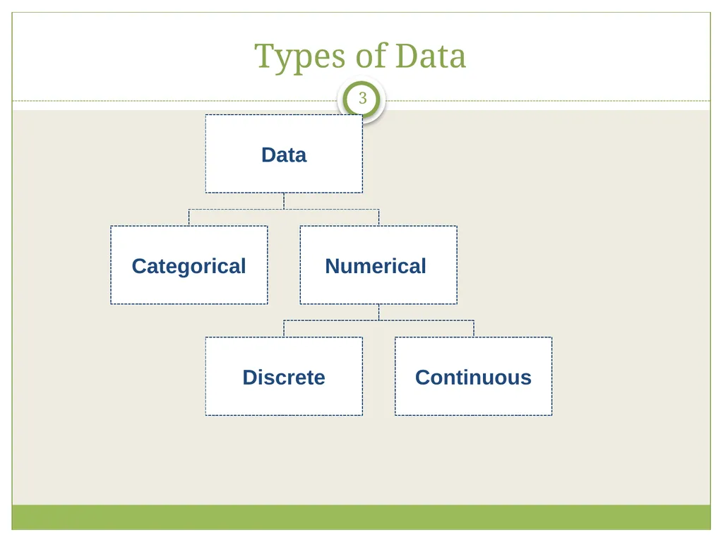
slide3. 3 Types of Data<br>
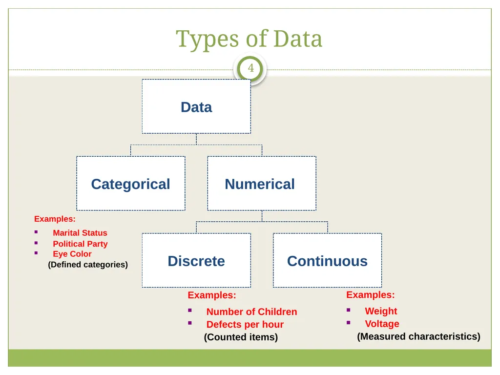
slide4. 4 Types of Data Examples:
Marital Status
Political Party
Eye Color
(Defined categories) Examples:
Number of Children
Defects per hour
(Counted items) Examples:
Weight
Voltage
(Measured characteristics)<br>
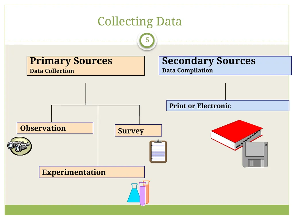
slide5. 5 Collecting Data Secondary Sources
Data Compilation Observation Experimentation Print or Electronic Survey Primary Sources
Data Collection<br>
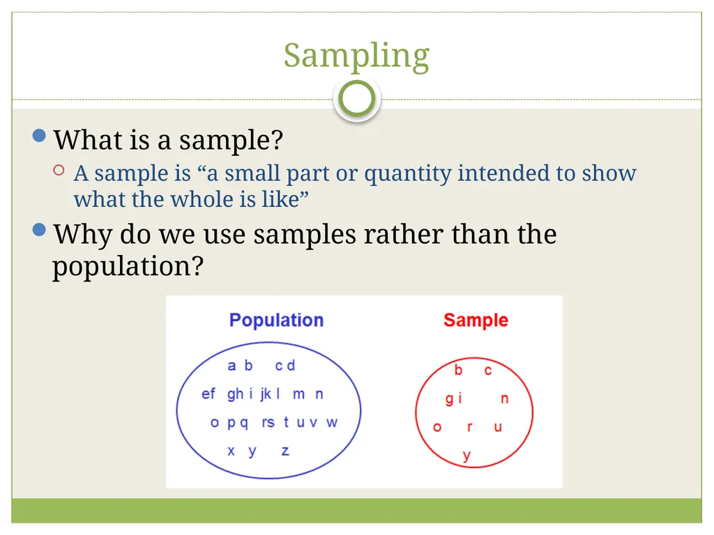
slide6. Sampling What is a sample?
A sample is “a small part or quantity intended to show what the whole is like”
Why do we use samples rather than the population?<br>
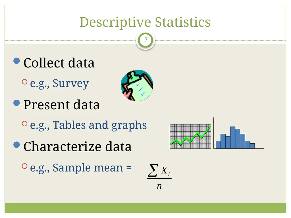
slide7. 7 Descriptive Statistics Collect data
e.g., Survey
Present data
e.g., Tables and graphs
Characterize data
e.g., Sample mean =<br>
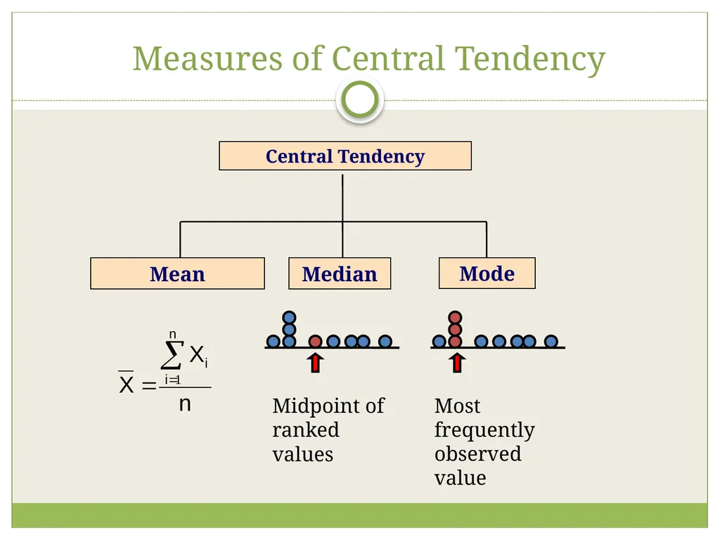
slide8. Measures of Central Tendency Central Tendency Mean Median Mode Midpoint of ranked values Most frequently observed value<br>
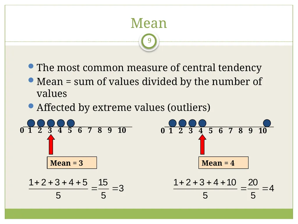
slide9. 9 Mean The most common measure of central tendency
Mean = sum of values divided by the number of values
Affected by extreme values (outliers) 0 1 2 3 4 5 6 7 8 9 10 Mean = 3 0 1 2 3 4 5 6 7 8 9 10 Mean = 4<br>
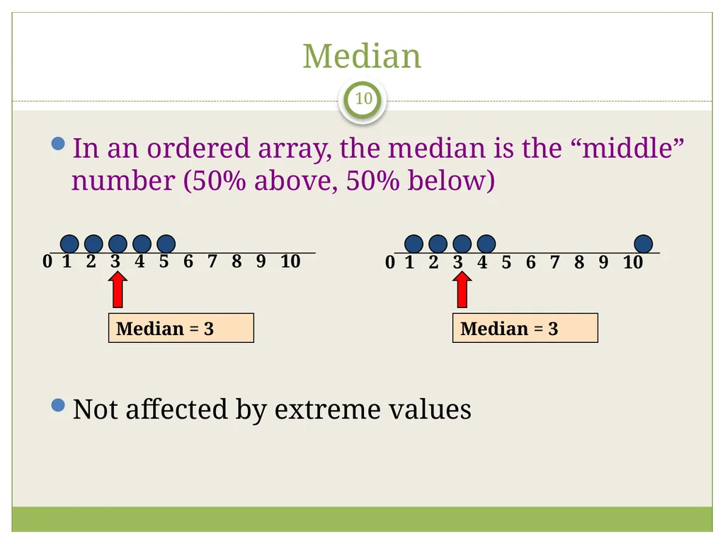
slide10. 10 Median In an ordered array, the median is the “middle” number (50% above, 50% below)
Not affected by extreme values 0 1 2 3 4 5 6 7 8 9 10 Median = 3 0 1 2 3 4 5 6 7 8 9 10 Median = 3<br>
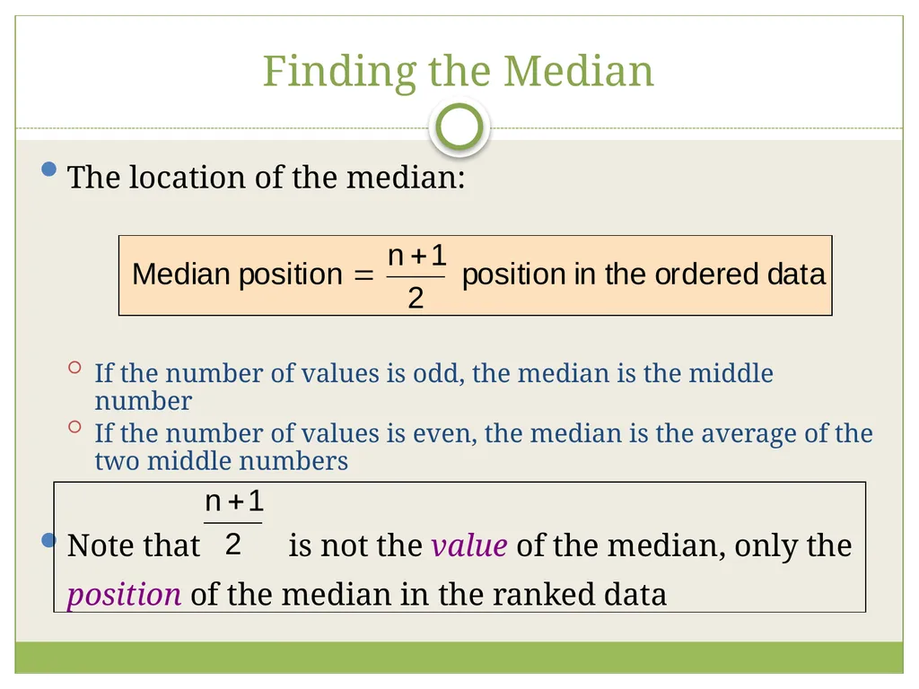
slide11. Finding the Median The location of the median:
If the number of values is odd, the median is the middle number
If the number of values is even, the median is the average of the two middle numbers
Note that is not the value of the median, only the position of the median in the ranked data<br>
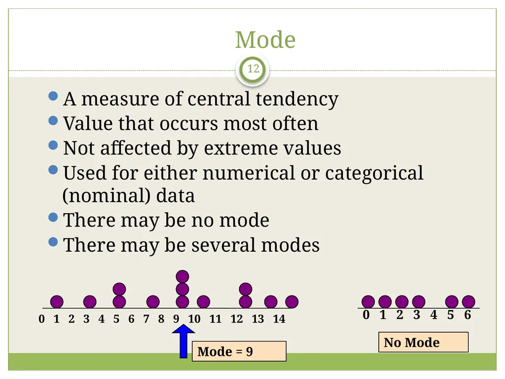
slide12. 12 Mode A measure of central tendency
Value that occurs most often
Not affected by extreme values
Used for either numerical or categorical (nominal) data
There may be no mode
There may be several modes 0 1 2 3 4 5 6 7 8 9 10 11 12 13 14 Mode = 9 0 1 2 3 4 5 6 No Mode<br>
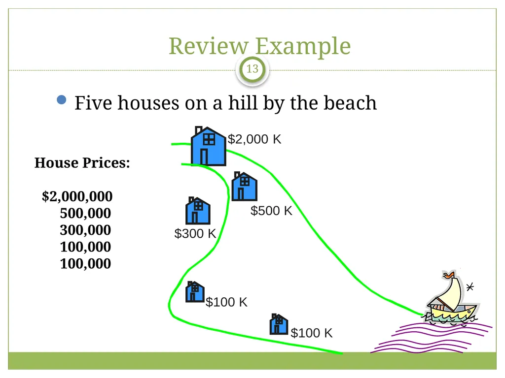
slide13. 13 Five houses on a hill by the beach Review Example House Prices: $2,000,000 500,000 300,000 100,000 100,000<br>
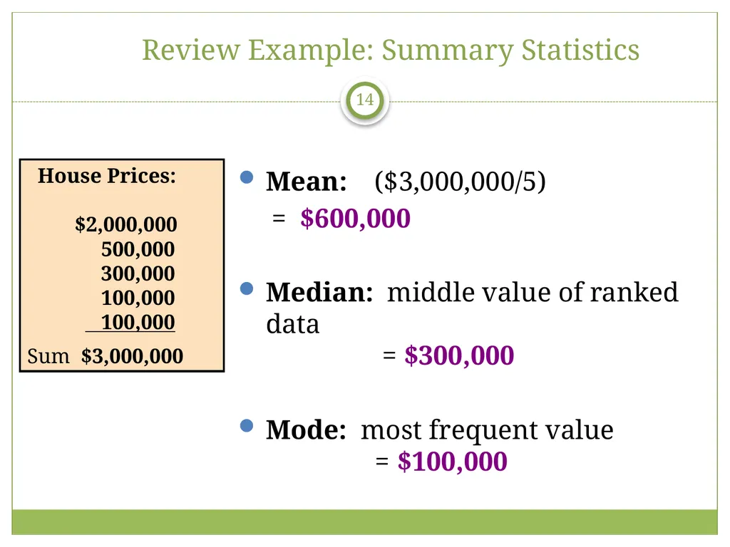
slide14. 14 Review Example: Summary Statistics Mean: ($3,000,000/5)
= $600,000
Median: middle value of ranked data = $300,000
Mode: most frequent value = $100,000 House Prices: $2,000,000
500,000 300,000 100,000 100,000
Sum $3,000,000<br>
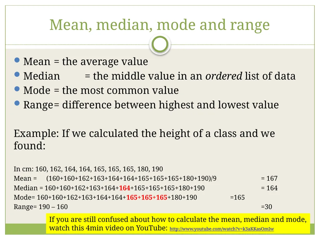
slide15. Mean, median, mode and range Mean = the average value
Median = the middle value in an ordered list of data
Mode = the most common value
Range = difference between highest and lowest value
Example: If we calculated the height of a class and we found:
In cm: 160, 162, 164, 164, 165, 165, 165, 180, 190
Mean = (160+160+162+163+164+164+165+165+165+180+190)/9 = 167
Median = 160+160+162+163+164+164+165+165+165+180+190 = 164
Mode= 160+160+162+163+164+164+165+165+165+180+190 =165
Range= 190 – 160 =30 If you are still confused about how to calculate the mean, median and mode,
watch this 4min video on YouTube: http://www.youtube.com/watch?v=k3aKKasOmIw<br>
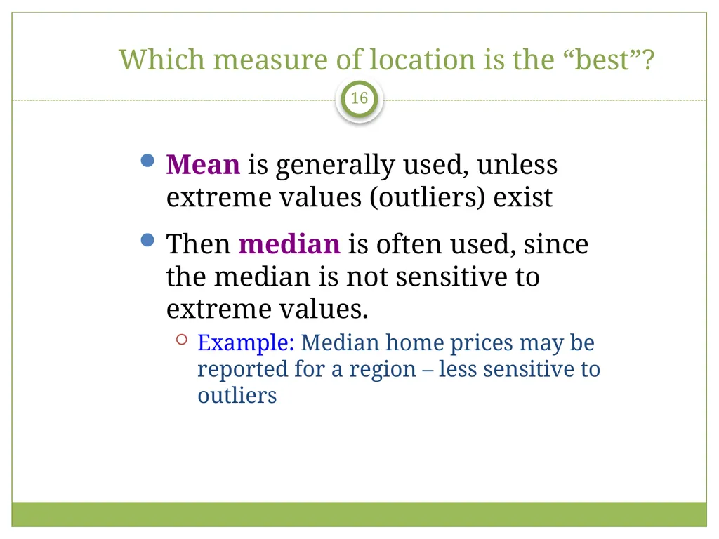
slide16. 16 Mean is generally used, unless extreme values (outliers) exist
Then median is often used, since the median is not sensitive to extreme values.
Example: Median home prices may be reported for a region – less sensitive to outliers Which measure of location is the “best”?<br>
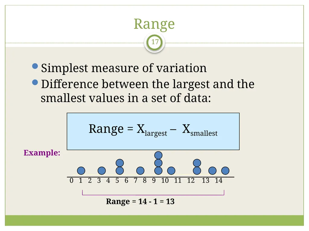
slide17. 17 Range Simplest measure of variation
Difference between the largest and the smallest values in a set of data: Range = Xlargest – Xsmallest 0 1 2 3 4 5 6 7 8 9 10 11 12 13 14 Range = 14 - 1 = 13 Example:<br>
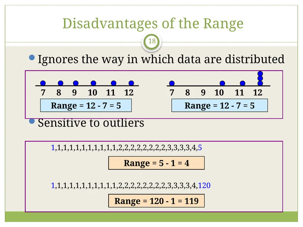
slide18. 18 Ignores the way in which data are distributed
Sensitive to outliers 7 8 9 10 11 12 Range = 12 - 7 = 5 7 8 9 10 11 12 Range = 12 - 7 = 5 Disadvantages of the Range 1,1,1,1,1,1,1,1,1,1,1,2,2,2,2,2,2,2,2,3,3,3,3,4,5 1,1,1,1,1,1,1,1,1,1,1,2,2,2,2,2,2,2,2,3,3,3,3,4,120 Range = 5 - 1 = 4 Range = 120 - 1 = 119<br>
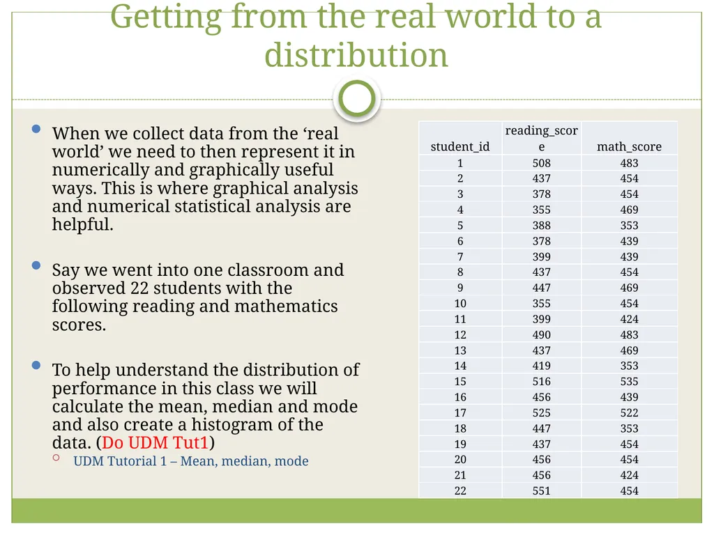
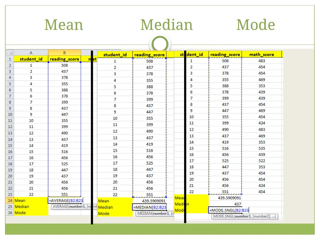
slide19. Getting from the real world to a distribution When we collect data from the ‘real world’ we need to then represent it in numerically and graphically useful ways. This is where graphical analysis and numerical statistical analysis are helpful.
Say we went into one classroom and observed 22 students with the following reading and mathematics scores.
To help understand the distribution of performance in this class we will calculate the mean, median and mode and also create a histogram of the data. (Do UDM Tut1)
UDM Tutorial 1 – Mean, median, mode<br>
slide20. Mean Median Mode<br>
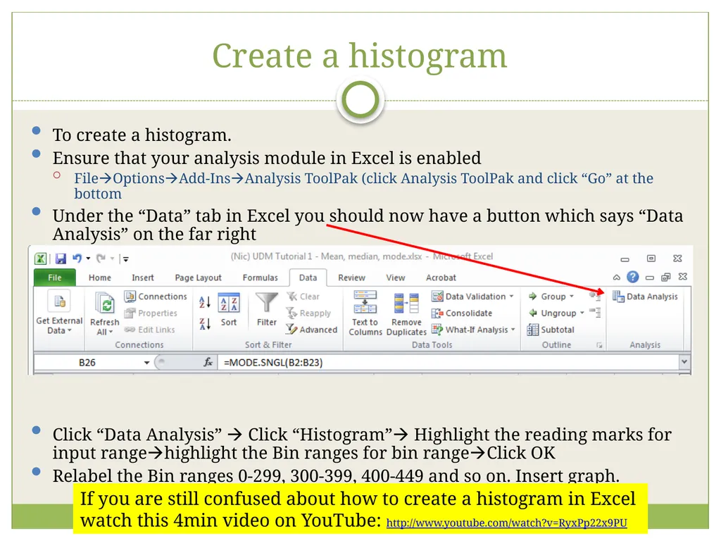
slide21. Create a histogram To create a histogram.
Ensure that your analysis module in Excel is enabled
FileOptionsAdd-InsAnalysis ToolPak (click Analysis ToolPak and click “Go” at the bottom
Under the “Data” tab in Excel you should now have a button which says “Data Analysis” on the far right
Click “Data Analysis” Click “Histogram” Highlight the reading marks for input rangehighlight the Bin ranges for bin rangeClick OK
Relabel the Bin ranges 0-299, 300-399, 400-449 and so on. Insert graph. If you are still confused about how to create a histogram in Excel
watch this 4min video on YouTube: http://www.youtube.com/watch?v=RyxPp22x9PU<br>
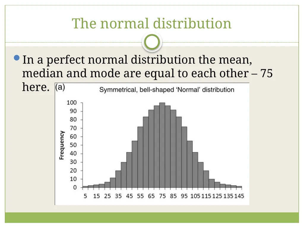
slide22. The normal distribution In a perfect normal distribution the mean, median and mode are equal to each other – 75 here.<br>
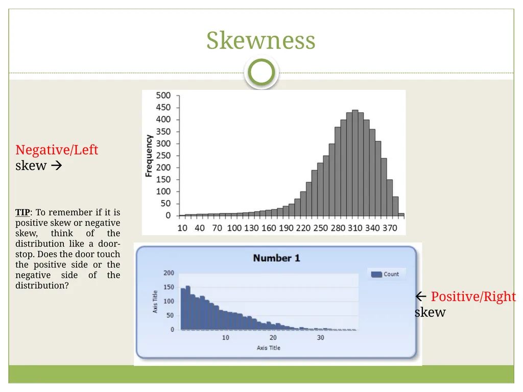
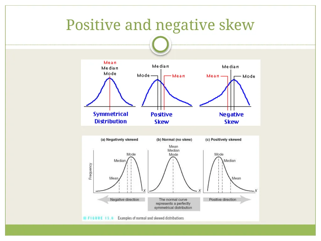
slide23. Skewness Negative/Left skew Positive/Right skew TIP: To remember if it is positive skew or negative skew, think of the distribution like a door-stop. Does the door touch the positive side or the negative side of the distribution?<br>
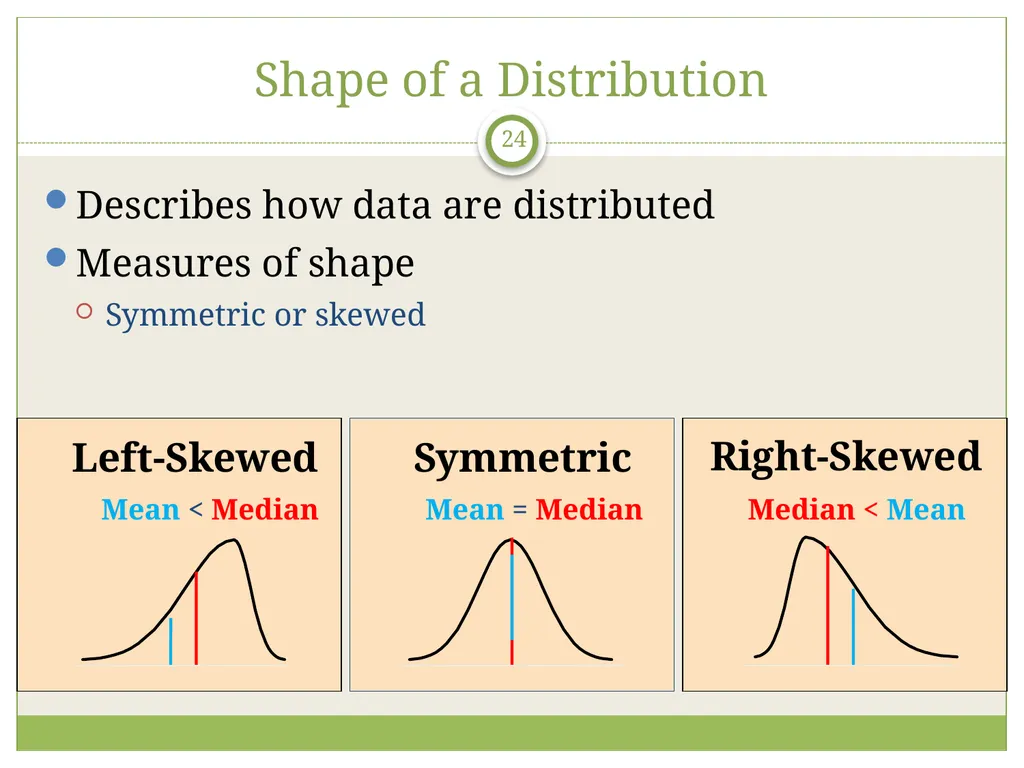
slide24. 24 Shape of a Distribution Describes how data are distributed
Measures of shape
Symmetric or skewed Mean = Median Mean < Median Median < Mean Right-Skewed Left-Skewed Symmetric<br>
slide25. Positive and negative skew<br>
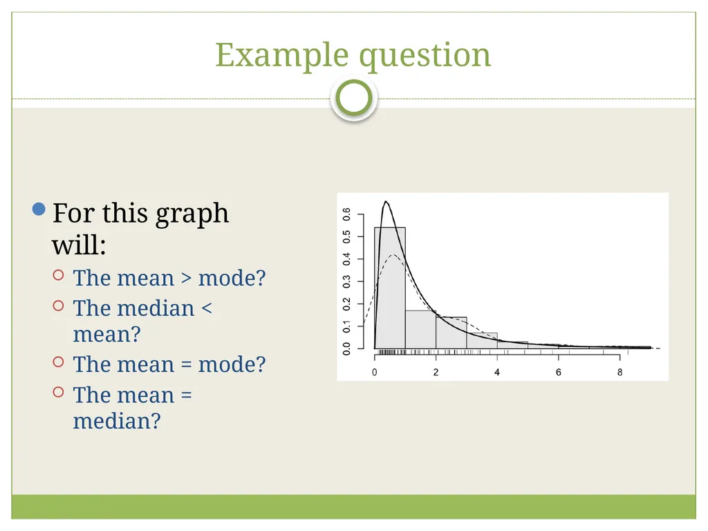
slide26. Example question For this graph will:
The mean > mode?
The median < mean?
The mean = mode?
The mean = median?<br>
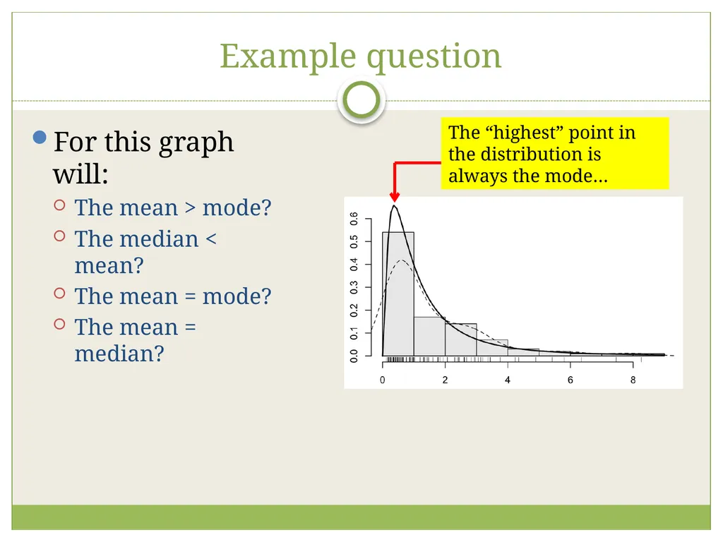
slide27. Example question For this graph will:
The mean > mode?
The median < mean?
The mean = mode?
The mean = median? The “highest” point in the distribution is always the mode…<br>
slide28. Tutorial quiz 1 Go to http://quizstar.4teachers.org/indexs.jsp
Enter your username and password
Click on “Basic Stats 101” Quiz and complete the quiz
If you have any questions raise your hand and I will come and help you
For those not already registered you can register as a student on http://quizstar.4teachers.org/indexs.jsp and then search for my class ”UDM Msc Education” anyone can join the class<br>
slide29. End of Lecture 1 For questions email me at NicholasSpaull@gmail.com
All slides/tutorials available at www.nicspaull.com/teaching<br>
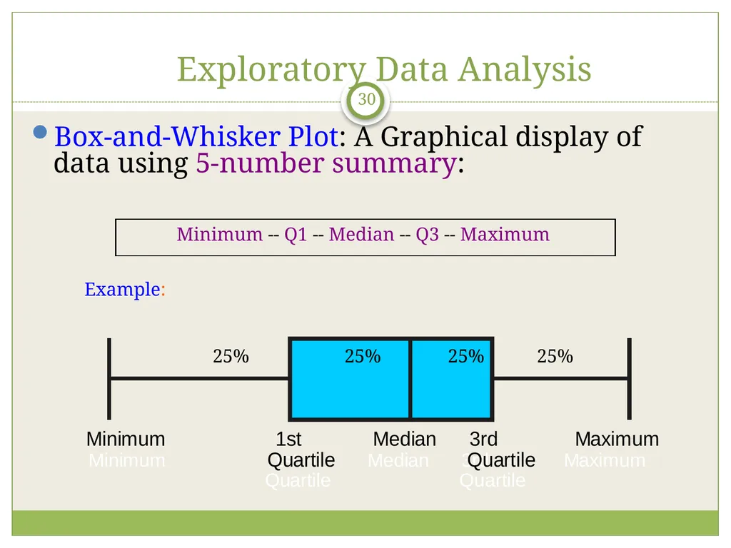
slide30. 30 Exploratory Data Analysis Box-and-Whisker Plot: A Graphical display of data using 5-number summary: Minimum -- Q1 -- Median -- Q3 -- Maximum Example: 25% 25% 25% 25%<br>
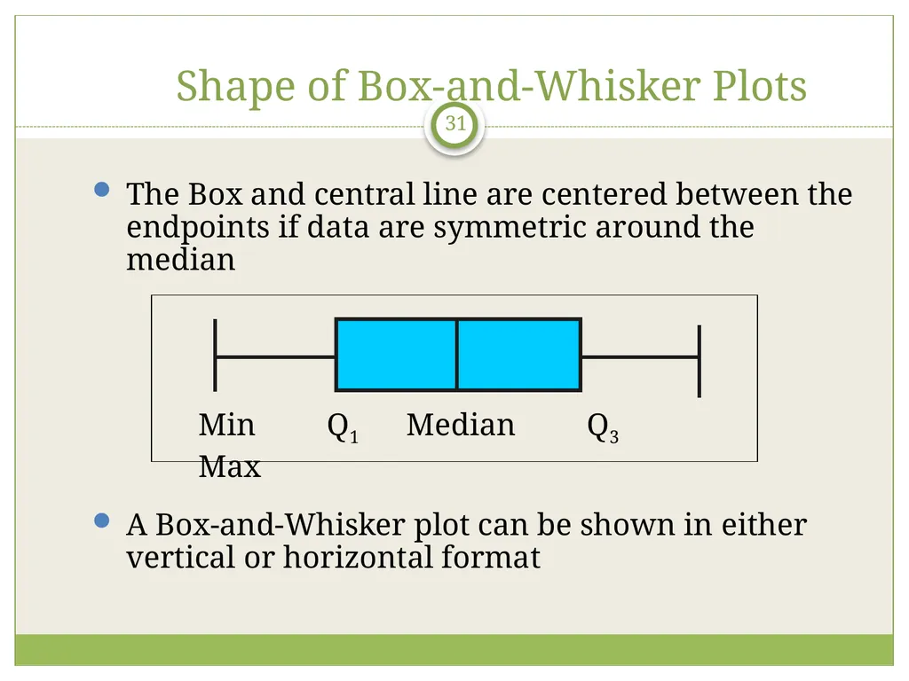
slide31. 31 Shape of Box-and-Whisker Plots The Box and central line are centered between the endpoints if data are symmetric around the median
A Box-and-Whisker plot can be shown in either vertical or horizontal format Min Q1 Median Q3 Max<br>
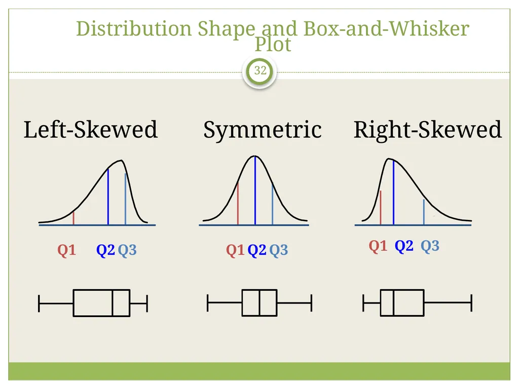
slide32. 32 Distribution Shape and Box-and-Whisker Plot Right-Skewed Left-Skewed Symmetric Q1 Q2 Q3 Q1 Q2 Q3 Q1 Q2 Q3<br>
2013
NicholasSpaull@gmail.com – www.nicspaull.com/teaching Day 2: Core statistics 101<br>
slide2. Introduction What are statistics?
“the practice or science of collecting and analysing numerical data in large quantities”
Why do we need descriptive statistics?
When we look at large amounts of data, there is very little “face value” information. If you had a dataset listing the income of 10,000 people and someone asked you if the income of the group was high or low it would be difficult to answer that question without using summary statistics (mean, median, mode etc.).<br>
slide3. 3 Types of Data<br>
slide4. 4 Types of Data Examples:
Marital Status
Political Party
Eye Color
(Defined categories) Examples:
Number of Children
Defects per hour
(Counted items) Examples:
Weight
Voltage
(Measured characteristics)<br>
slide5. 5 Collecting Data Secondary Sources
Data Compilation Observation Experimentation Print or Electronic Survey Primary Sources
Data Collection<br>
slide6. Sampling What is a sample?
A sample is “a small part or quantity intended to show what the whole is like”
Why do we use samples rather than the population?<br>
slide7. 7 Descriptive Statistics Collect data
e.g., Survey
Present data
e.g., Tables and graphs
Characterize data
e.g., Sample mean =<br>
slide8. Measures of Central Tendency Central Tendency Mean Median Mode Midpoint of ranked values Most frequently observed value<br>
slide9. 9 Mean The most common measure of central tendency
Mean = sum of values divided by the number of values
Affected by extreme values (outliers) 0 1 2 3 4 5 6 7 8 9 10 Mean = 3 0 1 2 3 4 5 6 7 8 9 10 Mean = 4<br>
slide10. 10 Median In an ordered array, the median is the “middle” number (50% above, 50% below)
Not affected by extreme values 0 1 2 3 4 5 6 7 8 9 10 Median = 3 0 1 2 3 4 5 6 7 8 9 10 Median = 3<br>
slide11. Finding the Median The location of the median:
If the number of values is odd, the median is the middle number
If the number of values is even, the median is the average of the two middle numbers
Note that is not the value of the median, only the position of the median in the ranked data<br>
slide12. 12 Mode A measure of central tendency
Value that occurs most often
Not affected by extreme values
Used for either numerical or categorical (nominal) data
There may be no mode
There may be several modes 0 1 2 3 4 5 6 7 8 9 10 11 12 13 14 Mode = 9 0 1 2 3 4 5 6 No Mode<br>
slide13. 13 Five houses on a hill by the beach Review Example House Prices: $2,000,000 500,000 300,000 100,000 100,000<br>
slide14. 14 Review Example: Summary Statistics Mean: ($3,000,000/5)
= $600,000
Median: middle value of ranked data = $300,000
Mode: most frequent value = $100,000 House Prices: $2,000,000
500,000 300,000 100,000 100,000
Sum $3,000,000<br>
slide15. Mean, median, mode and range Mean = the average value
Median = the middle value in an ordered list of data
Mode = the most common value
Range = difference between highest and lowest value
Example: If we calculated the height of a class and we found:
In cm: 160, 162, 164, 164, 165, 165, 165, 180, 190
Mean = (160+160+162+163+164+164+165+165+165+180+190)/9 = 167
Median = 160+160+162+163+164+164+165+165+165+180+190 = 164
Mode= 160+160+162+163+164+164+165+165+165+180+190 =165
Range= 190 – 160 =30 If you are still confused about how to calculate the mean, median and mode,
watch this 4min video on YouTube: http://www.youtube.com/watch?v=k3aKKasOmIw<br>
slide16. 16 Mean is generally used, unless extreme values (outliers) exist
Then median is often used, since the median is not sensitive to extreme values.
Example: Median home prices may be reported for a region – less sensitive to outliers Which measure of location is the “best”?<br>
slide17. 17 Range Simplest measure of variation
Difference between the largest and the smallest values in a set of data: Range = Xlargest – Xsmallest 0 1 2 3 4 5 6 7 8 9 10 11 12 13 14 Range = 14 - 1 = 13 Example:<br>
slide18. 18 Ignores the way in which data are distributed
Sensitive to outliers 7 8 9 10 11 12 Range = 12 - 7 = 5 7 8 9 10 11 12 Range = 12 - 7 = 5 Disadvantages of the Range 1,1,1,1,1,1,1,1,1,1,1,2,2,2,2,2,2,2,2,3,3,3,3,4,5 1,1,1,1,1,1,1,1,1,1,1,2,2,2,2,2,2,2,2,3,3,3,3,4,120 Range = 5 - 1 = 4 Range = 120 - 1 = 119<br>
slide19. Getting from the real world to a distribution When we collect data from the ‘real world’ we need to then represent it in numerically and graphically useful ways. This is where graphical analysis and numerical statistical analysis are helpful.
Say we went into one classroom and observed 22 students with the following reading and mathematics scores.
To help understand the distribution of performance in this class we will calculate the mean, median and mode and also create a histogram of the data. (Do UDM Tut1)
UDM Tutorial 1 – Mean, median, mode<br>
slide20. Mean Median Mode<br>
slide21. Create a histogram To create a histogram.
Ensure that your analysis module in Excel is enabled
FileOptionsAdd-InsAnalysis ToolPak (click Analysis ToolPak and click “Go” at the bottom
Under the “Data” tab in Excel you should now have a button which says “Data Analysis” on the far right
Click “Data Analysis” Click “Histogram” Highlight the reading marks for input rangehighlight the Bin ranges for bin rangeClick OK
Relabel the Bin ranges 0-299, 300-399, 400-449 and so on. Insert graph. If you are still confused about how to create a histogram in Excel
watch this 4min video on YouTube: http://www.youtube.com/watch?v=RyxPp22x9PU<br>
slide22. The normal distribution In a perfect normal distribution the mean, median and mode are equal to each other – 75 here.<br>
slide23. Skewness Negative/Left skew Positive/Right skew TIP: To remember if it is positive skew or negative skew, think of the distribution like a door-stop. Does the door touch the positive side or the negative side of the distribution?<br>
slide24. 24 Shape of a Distribution Describes how data are distributed
Measures of shape
Symmetric or skewed Mean = Median Mean < Median Median < Mean Right-Skewed Left-Skewed Symmetric<br>
slide25. Positive and negative skew<br>
slide26. Example question For this graph will:
The mean > mode?
The median < mean?
The mean = mode?
The mean = median?<br>
slide27. Example question For this graph will:
The mean > mode?
The median < mean?
The mean = mode?
The mean = median? The “highest” point in the distribution is always the mode…<br>
slide28. Tutorial quiz 1 Go to http://quizstar.4teachers.org/indexs.jsp
Enter your username and password
Click on “Basic Stats 101” Quiz and complete the quiz
If you have any questions raise your hand and I will come and help you
For those not already registered you can register as a student on http://quizstar.4teachers.org/indexs.jsp and then search for my class ”UDM Msc Education” anyone can join the class<br>
slide29. End of Lecture 1 For questions email me at NicholasSpaull@gmail.com
All slides/tutorials available at www.nicspaull.com/teaching<br>
slide30. 30 Exploratory Data Analysis Box-and-Whisker Plot: A Graphical display of data using 5-number summary: Minimum -- Q1 -- Median -- Q3 -- Maximum Example: 25% 25% 25% 25%<br>
slide31. 31 Shape of Box-and-Whisker Plots The Box and central line are centered between the endpoints if data are symmetric around the median
A Box-and-Whisker plot can be shown in either vertical or horizontal format Min Q1 Median Q3 Max<br>
slide32. 32 Distribution Shape and Box-and-Whisker Plot Right-Skewed Left-Skewed Symmetric Q1 Q2 Q3 Q1 Q2 Q3 Q1 Q2 Q3<br>