MODELING COMMANDS CHAPTER 11Whenever you see this prompt,is ready to r - PDF document

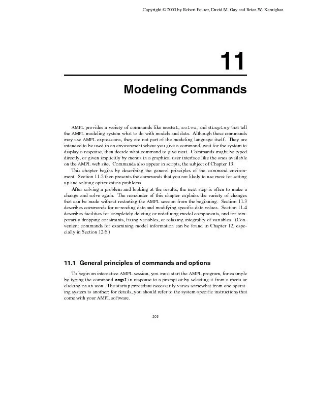
MODELING COMMANDS CHAPTER 11Whenever you see this prompt,is ready to read and interpret what you type. Ascommand ends with a semicolon. If you enter one or more complete com-prompt again. If you end a line in the middle of a command, you areprompted to continue it on the next line; you can tell thatit on the next line; you can tell thatYou can type any number of characters on a line (up to whatever limit your operating sys-Several commands use filenames for reading or writing information. A filename cansequence of any characters enclosed in matching quotes. The rules for correct filenames. For the examples in thisfrom a graphical interface, the details of your interactionwill be different, but the command interface is likely to be accessible, and in fact is beingcommands depends not only on what you type directly, but ona variety of options for choosing alternative solvers, controlling the display of results, andEach option has a name, and a value that may be a number or a character string. Forare strings that specify the prompts. Thehas a numeric value, which says how many characters widecommand displays and sets option values. If SECTION 11.1 GENERAL PRINCIPLES OF COMMANDS AND OPTIONSis followed by a name and a value, it resets the named option to thespecified value. In the following example we change the prompt and the display width,You can specify any string value by surrounding the string in matching quotesas above; the quotes may be omitted if the string looks like a name or number.) denote an empty string, which is a meaningful valuefor some options. At the other extreme, if you want to spread a long string over severalstarts, it sets many options to initial, or default, values. The, for instance, so prompts appear in the standard way.option has a default value of 79. Other options, especially onesyou define. Thus if you mis-type an option name, you will most likely define a newstatement also doesn’t check to see if you have assigned a meaningful valueto an option. You will be informed of a value error only when an option is used by somesubsequent command. In these respects,options are much like operating system orshell ‘‘environment variables.’’ In fact you can use the settings of environment variables MODELING COMMANDS CHAPTER 1111.2 Setting up and solving models and dataTo apply a solver to an instance of a model, the examples in this book usecommand names a file that contains model declarations (Chapters 5 through(Chapter 9). Thecommand causes a description of the optimization problem tobe sent to a solver, and the results to be retrieved for examination. This section takes afeatures for setting up and solving models. Features formaintains a ‘‘current’’ model, which is the one that will be sent to the solver if. At the beginning of an interactive session, the current model is empty.command reads declarations from a file and adds them to the current model; acommand reads data statements from a file to supply values for componentsalready in the current model. Thus you may use severalbuild up the description of an optimization problem, reading different parts of the modelYou can also type parts of a model and its data directly at annents to the current model. The data statements of Chapter 9 also act as commands,which supply data values for already defined components such as sets and parameters.Because model and data statements look much alike, however, you need to tellalways starts out in ‘‘model mode’’; the statement(without a filename) switches the interpreter to ‘‘data mode’’, and the statement(without a filename) switches it back. Any command (like) that does not begin like a data statement also has the effect of switchingIf a model declares more than one objective function,them to the solver. Most solvers deal only with one objective function and usually selectthe first by default. TheIf a model has an indexed collection of objectives, you must supply a subscript to indicate SECTION 11.2 SETTING UP AND SOLVING MODELS AND DATAcommand sets in motion a series of activities. First, it causesgenerate a specific optimization problem from the model and data that you have supplied.If you have neglected to provide some needed data, an error message is printed; you willalso get error messages if your data values violate any restrictions imposed by qualifica-, because a restriction may depend in a compli-cated way on many different data values. Arithmetic errors like dividing by zero are alsoAfter the optimization problem is generated,tries to make the problem easier for the solver. Sometimes presolve so greatly reducesthe size of a problem that it become substantially easier to solve. Normally the work ofpresolve goes on behind the scenes, however, and you need not be concerned about it. Inrare cases, presolve can substantially affect the optimal values of the variables — whenthere is more than one optimal solution — or can interfere with other preprocessing rou-tines that are built into your solver software. Also presolve sometimes detects that nofeasible solution is possible, and so does not bother sending your program to the solver.For example, if you drastically reduce the availability of one resource inreduce the availability of one resource inampl:solve;presolve: constraint Time[’reheat’] cannot hold:&#x= 10;&#x can;&#xnot ;¾ 0;body For these cases you should consult the detailed description of presolve in Section 14.1.The generated optimization problem, as possibly modified by presolve, is finally sentto the solver of your choice. Every version ofdefault solver that will be used automatically if you give no other instructions; typeIf you have more than one solver, you can switch among them by changing the MODELING COMMANDS CHAPTER 11In this example we reset the problem between solves, so that the solvers are invoked withthe same initial conditions and their performance can be compared. Without reset, infor-mation about the solution found by one solver would be passed along to the next one,possibly giving the latter a substantial advantage. Passing information from oneto the next is most useful when a series of similar LPs are to be sent to the same solver;Almost any solver can handle a linear program, although those specifically designedfor linear programming generally give the best performance. Other kinds of optimizationproblems, such as nonlinear (Chapter 18) and integer (Chapter 20), can be handled onlyby solvers designed for them. A message such as ‘‘ignoring integrality’’ or ‘‘can’t han-dle nonlinearities’’ is an indication that you have not chosen a solver appropriate for yourIf your optimization problems are not too difficult, you should be able to usewithout referring to instructions for a specific solver: set theIf your solver takes a very long time to return with a solution, or returns towithout any ‘‘optimal solution’’ message, then it’s time to read further. Each solver is asophisticated collection of algorithms and algorithmic strategies, from which many com-binations of choices can be made. For most problems the solver makes good choicesautomatically, but you can also pass along your own choices throughdetails may vary with each solver, so for more information you must look to the solver-If your problem takes a long time to optimize, you will want some evidence of thesolver’s progress to appear on your screen. Directives for this purpose are also described SECTION 11.3 MODIFYING DATA11.3 Modifying databy somewhat different data. We describe here’s facilities for resetting parametervalues while leaving the model as is. They include commands for resetting data modeTo delete the current data for several model components, without changing the currentcommands to read in new values for these sets and parameters.command works similarly, but does not actually delete any datauntil new values are assigned. Thus if you typewill remain. If instead you usedwould be without values, and you would get an error message when you nextdescribed in Section 7.6. Continuing with the variant ofis changed so that its value is given byby)with corresponding data:param avail_mean := reheat 35 roll 40 ;param avail_variance := reheat 5 roll 2 ;thenAMPLwill take new samples from theNormaldistribution after eachresetdata. Different samples result in different solutions, and hence in different optimal MODELING COMMANDS CHAPTER 11roll 43.038 ;roll 32.6855 ;repeat from the beginning. (Sectioncommand also permits you to change particular data values while leaving. You can use it, for example, to solve the diet model ofFigure 5-1, trying out a series of upper bounds SECTION 11.3 MODIFYING DATAis made for each member of the specified indexing set. You could use this feature totoor to increase all upper bounds by 10 percent:let {j in FOOD} f_max[j] := 1.1 * f_max[j];In general this command consists of the keywordlet, an indexing expression if needed,and an assignment. Any set or parameter whose declaration does not define it using anphrase may be specified to the left of the assignment’sdoes not impose any restrictions on what you can change usingyou should take care in changing any set or parameter that affects the indexing of otherFor example, after solving the multiperiod production problem of Figures 4-4 and 4-5,4-5,error processing param market:2 invalid subscripts discarded:market[’bands’,4]market[’coils’,4]error processing param revenue:2 invalid subscripts discarded:revenue[’bands’,4]revenue[’coils’,4]error processing var Sell[’coils’,1]:invalid subscript market[’bands’,4]The problem here is thatAMPLstill has current data for 4th-week parameters such ascurrent data for 4th-week parameters such as, which has become invalid with the change ofto 3. If you want to properlyreduce the number of weeks in the linear program while using the same data, you mustcommand to change the current values of variables. This issometimes a convenient feature for exploring an alternative solution. For example, here MODELING COMMANDS CHAPTER 11is what happens when we solve for the optimal diet as above, then round the optimalwe solve for the optimal diet as above, then round the optimal()ampl:display Total_Cost, n_min, Diet_Min.slack;;Total_Cost = 70.8: n_min Diet_Min.slack :=A 700 231C 700 -40CAL 16000 -640slacks are automatically computed from the new, rounded values. The cost has droppedprovides a variety of rounding functions that can be used in this way. They are11.4 Modifying modelsSeveral commands are provided to help you make limited changes to the currentmodel, without modifying the model file or issuing a full. This section describescommands that completely remove or redefine model components, and that temporarily SECTION 11.4 MODIFYING MODELSthat no other components use it in their declarations. The form of the command is simplyNormally you cannot delete a set, parameter, or variable, because it is declared for uselater in the model; but you can delete any objective or constraint. You can also specify a. It removes not only the listed components, but also all components thaton them either directly (by referring to them) or indirectly (by referring to their depen-dents). Thus for example inThus for example in�var Buy {j in FOOD} = f_min[j], minimize Total_Cost: sum {j in FOOD} cost[j] * Buy[j];. It also deletesthrough its reference toIf you’re not sure which components depend on some given component, you can usecommand can be applied to any list of model com-Once a component has been removed bymeaning of the component’s name becomes visible again. After a constraint namedIf there is no previously hidden meaning, the name of a component removed bybecomes again unused, and may subsequently be declared as thename of any new component of any type. If you only want to make some relatively lim-ited modifications to a declaration, however, then you will probably findbe more convenient. You can change any component’s declaration by writing the key- MODELING COMMANDS CHAPTER 11substitute. Looking again at. The declarations of all components thatA list of all component types to whichThe simplest (but most drastic) way to change the model is by issuing the command, which expunges all of the current model and data. Followingtheir default values. If your operating system or your graphical environment forallows you to edit files while keepingexperimentation; you may make changes to the model or data files, typeread in the modified files. (If you need to escape fromcurrent model. As an example, the constraints of Figure 5-1 initially includeAs an example, the constraints of Figure 5-1 initially includeAdropcommand can specify a particular one of these constraints to ignore:drop Diet_Max["CAL"];or it may specify all constraints or objectives indexed by some set:drop {i in MAXNOT} Diet_Max[i];whereMAXNOThas previously been defined as some subset ofMAXREQ. The entire col-The entire col-or more simply:drop Diet_Max;In general, this command consists of the keyworddrop, an optional indexing expression,and a constraint name that may be subscripted. Successivecommand reverses the effect of. It has the same syntax, except SECTION 11.4 MODIFYING MODELScommand fixes specified variables at their current values, as if there were aconstraint that the variables must equal these values; theeffect. These commands have the same syntax asname variables rather than constraints. For example, here we initialize all variables ofour diet problem to their lower bounds, fix all variables representing foods that have moremoreampl:�fix {j in FOOD: amt["NA",j] 1200} Buy[j];ampl:solve;MINOS 5.5: optimal solution found.7 iterations, objective 86.92Objective = Total_Cost[’A&P’]ampl:display {j in FOOD} (Buy[j].lb,Buy[j],amt["NA",j]);: Buy[j].lb Buy[j] amt[’NA’,j] :=BEEF 2 2 938CHK 2 2 2180FISH 2 10 945HAM 2 2 278MCH 2 9.42857 1182MTL 2 10 896SPG 2 2 1329TUR 2 2 1397Rather than setting and fixing the variables in separate statements, you can add an assign-�assign-Theunfixcommand works in the same way, to reverse the effect of fix and optionallyto ignore all restrictions of variables to integer values. Variables declaredget whatever bounds you specified for them, while variables declaredare given a lower bound of zero and an upper bound of one. To restore the inte-relaxation status: 0 if integrality is enforced, nonzero otherwise. You can make use ofthis suffix to relax integrality on selected variables only. For example, MODELING COMMANDS CHAPTER 11�11relaxes integrality on allBuyvariables for foods that have a minimum purchase of atSome of the solvers that work withintegrality, but these do not necessarily have the same effect assuffix. The distinction is due to the effects’s problem simplification, or presolve, stage (Section 14.1).the presolve phase, so that the solver receives a true continuousrelaxation of the original integer problem. If the relaxation is performed by the solver,however, then the integrality restrictions are still in effect duringAs a simple example, suppose that diet model variable declarations are written tosimple example, suppose that diet model variable declarations are written toIn our example of Figure 2-3, all of theto 0.95. First, here are the results of solving the unrelaxed problem:When no relaxation is specified inlimits of 9.5, and since it knows that the variables must take integer values, it roundsthese limits down to 9. Then these limits are sent to the solver, where they remain even if SECTION 11.4 MODIFYING MODELSis set to 1, presolve leaves the upper limits at9.5 and sends those to the solver, with the result being a less constrained problem andandBEEF 6.8798CHK 2FISH 2HAM 9.5MCH 9.5MTL 9.5SPG 9.1202TUR 2;Variables that were at upper bound 9 in the previous solution are now at upper bound 9.5.The same situation can arise in much less obvious circumstances, and can lead tounexpected results. In general, the optimal value of an integer program underoption may be lower (for minimization) or higher (for maxi- modeling system what to do with models and data. Although these commandsexpressions, they are not part of the modeling language itself. They aredisplay a response, then decide what command to give next. Commands might be typedweb site. Commands also appear in scripts, the subject of Chapter 13.ment. Section 11.2 then presents the commands that you are likely to use most for settingAfter solving a problem and looking at the results, the next step is often to make achange and solve again. The remainder of this chapter explains the variety of changessession from the beginning. Section 11.3describes commands for re-reading data and modifying specific data values. Section 11.4describes facilities for completely deleting or redefining model components, and for tem-porarily dropping constraints, fixing variables, or relaxing integrality of variables. (Con-venient commands for examining model information can be found in Chapter 12, espe-11.1 General principles of commands and optionsclicking on an icon. The startup procedure necessarily varies somewhat from one operat-ing system to another; for details, you should refer to the system-specific instructions that