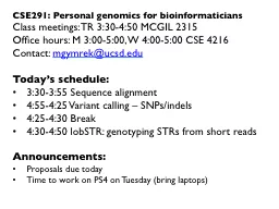
bioinformaticians Class meetings TR 330450 MCGIL 2315 Office hours M 300500 W 400500 CSE 4216 Contact mgymrekucsdedu Todays schedule 330 355 Sequence alignment 4 55 ID: 795960
Download The PPT/PDF document "CSE291: Personal genomics for" is the property of its rightful owner. Permission is granted to download and print the materials on this web site for personal, non-commercial use only, and to display it on your personal computer provided you do not modify the materials and that you retain all copyright notices contained in the materials. By downloading content from our website, you accept the terms of this agreement.
Slide1
CSE291: Personal genomics for
bioinformaticians
Class meetings: TR 3:30-4:50 MCGIL 2315
Office hours: M 3:00-5:00, W 4:00-5:00 CSE 4216
Contact:
mgymrek@ucsd.edu
Today’s schedule:
3:30
-
3:55
Sequence alignment
4
:55-
4
:25
Variant calling – SNPs/indels
4:
25-
4
:
30
Break
4
:
30
-
4:50
lobSTR
: genotyping STRs from short reads
Announcements
:
Proposals due today
Time to work on PS4 on Tuesday (bring laptops)
Slide2Short read alignment and variant calling
CSE291: Personal Genomics for
Bioinformaticians
02/
16/
17
Slide3Outline
Mapping using BWT
Local realignment
Basic SNP calling approaches
State of the art variant calling
Genotyping STRs from short reads
Slide4Mapping using BWT
Slide5The data! – “FASTQ”
ERR194146_1.fastq
@ERR194146.1 HSQ1008:141:D0CC8ACXX:3:1308:20201:36071/1
ACATCTGGTTCCTACTTCAGGGCCATAAAGCCTAAATAGCCCACACGTTCCCCTTAAATAAGACATCACGATGGATCACAGGTCTATCACCCTATTAACCA
+
?@@FFBFFDDHHBCEAFGEGIIDHGH@GDHHHGEHID@C?GGDG@FHIGGH@FHBEG:GGIEEHH;@CHH=EDFFBBE>;@?3;;;>;;;AA?<C>C@@C:
@ERR194146.2 HSQ1008:141:D0CC8ACXX:4:1208:5231:93701/1
CCAGCGTCTCGCAATGCTATCGCGTGCATACCCCCCAGACGAAAATACCAAATGCATGGAGAGCTCCCGTGAGTGGTTAATAGGGTGATAGACCTGTGATC
+
?88ADA?BDF8F:@@DB49C>B7C806B<?DEF=@FFC=AABEA<;@D>AC265;ADA;@@?<@B@A<;?5(8+:0>(4:@AAA832?@@BBBB:<4(:>>
@ERR194146.3 HSQ1008:141:D0CC8ACXX:2:1305:18078:8420/1GATCACAGGTCTATCACCCTATTAACCACTCACGGGAGCTCTCCATGCATTTGGTATTTTCGTCTGGGGGGTATGCACGCGATAGCATTGCGAGACGCTGG+@CCFFFFFHHFGHJIGJJJJJJJJJJJIJIIJJJIJJJIGJJJJIIJIGIHIJI=FFIJJJJHHJHGHHDD;@CDDEDDDDDBDDDCECDDDDDBDDDDDD
ERR194146_2.fastq
@ERR194146.1 HSQ1008:141:D0CC8ACXX:3:1308:20201:36071/2CCAGCGTCTCGCAATGCTATCGCGTGCATACCCCCCAGACGAAAATACCAAATGCATGGAGAGCTCCCGTGAGTGGTTAATAGGGTGATAGACCTGTGATC+<?@DDDBDHHHAAH@CG@FBBGGIEG@D@GCHFG@F/5=C4=B'=7?CA9@?ACDCDCA@<?BDCCCB=BB0<4>?4?>@:CCD???A:@C3>A>AC:++:@ERR194146.2 HSQ1008:141:D0CC8ACXX:4:1208:5231:93701/2CCCACACGTTCCCCTTAAATAAGACATCACGATGGATCACAGGTCTATCACCCTATTAACCACTCACGGGAGCTCTCCATGCATTTGGTATTTTCGTCTGG+@??BD1:AFHBDDGGHIJIF@EEE>GFHGHEAG?DEG<FD>B;?BB<*/9??C8BB@FHC7=CCGAE;=,5,,.;@@>(5(;>ACCC(,,5;>CCB88<??@ERR194146.3 HSQ1008:141:D0CC8ACXX:2:1305:18078:8420/2GATCACAGGTCTATCACCCTATTAACCACTCACGGGAGCTCTCCATGCATTTGGTATTTTCGTCTGGGGGGTATGCACGCGATAGCATTGCGAGACGCTGG+@CCFFFFFHHFGHJIGJJJJJJJJJJJIJIIJJJIJJJIGJJJJIIJIGIHIJI=FFIJJJJHHJHGHHDD;@CDDEDDDDDBDDDCECDDDDDBDDDDDD
(first end of each pair)
(second end of each pair)
Slide6Challenge: Rapidly align short reads to a reference
Goal:
Where in the genome does each read originate?
Reference genome: ~3×10
9
bp
Reads: ~100bp
Solution:
Index genome in quickly searchable data structure
Genome
Index
?
(Burrows Wheeler Transform)
ACGATAG
Chr1:3899292
ATCGACGATAGCCG
ACGATAG
Slide7Burrows-Wheeler Transform
String T
:
AACATCGAGCTACGTACGTACGTACGTACGTACGTACGTACGACGAGGGGAGAGAAT
BWT(T)
(Burrows Wheeler Transform
)
Size O(|T|), searching in time O(|query string|)
T
Burrows Wheeler Transform (and related auxiliary data structures) allows:
Compression
Indexing/searching
Slide8Burrows-Wheeler Transform
String T: BANANA$
m
=|T| (length of T)
T ends with a terminator character ($), lexicographically prior to all other characters
Creating BWT(T)
Write down rotations of T
Sort the rows lexicographically to make BWM(T) (Burrows Wheeler Matrix)
The final column of BWM(T) gives BWT(T)
Step 1:
B A N A N A
$$ B A N A N AA
$ B A N A NN A $ B A N AA N A $ B A NN A N A $ B AA N A N A $ BStep 2:$ B A N A N AA
$ B A N A NA N A $
B A N
A N A N A
$
B
B A N A N A
$
N A
$
B A N A
N A N A
$
B A
BWT(T) = ANNB$AA
Slide9Relationship to suffix arrays
String T: BANANA$
Creating
SuffixArray
(T)
Write T’s suffixes, note the starting index of each suffix
Sort lexicographically
BWM(T)
SuffixArray
(T)
Suffix given by SA
$ B A N A N A
A $ B A N A NA N A $ B A NA N A N A $ BB A N A N A $N A $ B A N AN A N A $ B A$ A $A N A
$A N A N A
$
B A N A N A
$
N A
$
N A N A
$
6
5
3
1
04
2BWT(T)[i
] =
T[SA[i]-1] if SA[i
]>0
$ if SA[i
]==0
Slide10BWT for compression
BWT is
reversible
, necessary for compression
BWT(T) has same length as T, so not immediately clear where compression comes in.
BUT BWT often brings similar characters together, easier to shrink with run length encoding methods, e.g. bzip2
BWT(BANANA$) =
ANNB$AA
BWT(tomorrow and tomorrow and tomorrow) =
wwwdd
nnoooaatttmmmrrrrrrooo $
ooo
Slide11Reversing the BWT with LF mapping
Step 1:
B
0
A
0
N
0
A
1
N1 A2 $0$0
B0 A0
N0 A1 N1 A2A2 $0 B0 A0 N0 A1 N1
N1 A2
$
0
B
0
A
0
N
0
A
1A1 N1
A2 $0
B
0 A0 N0
N0
A1 N
1 A2 $
0
B0
A0A0
N0 A1
N
1
A
2
$
0
B
0
Step 2:
Create the BWM, but this time include order of each character
e.g.:
B
0
A
0
N
0
A
1
N
1
A
2
$
$
0
B
0
A
0
N
0
A
1
N
1
A
2
A
2
$
0
B0 A0 N0 A1 N1A1 N1 A2 $0 B0 A0 N0A0 N0 A1 N1 A2 $0 B0B0 A0 N0 A1 N1 A2 $0N1 A2 $0 B0 A0 N0 A1N0 A1 N1 A2 $0 B0 A0
LF Property
: the
i
th
occurrence of a character
c
in the last column (L) has the same rank as the
i
th
occurrence of
c
in the first column (F)
e.g. for A, has order 2, 1, 0 in both L and F
e.g. for N, has order 1, 0 in both L and F
Slide12Reversing the BWT with LF mapping
T =
B
0
A
0
N
0
A
1
N1 A2 $$0
B0 A0 N0
A1 N1 A2A2 $0 B0 A0 N0 A1 N1A
1 N1 A
2
$
0
B
0
A
0
N
0
A0 N0 A1
N1 A2
$0
B0B
0 A0
N0 A
1 N1 A2
$
0N
1 A2 $
0 B0
A
0
N
0
A
1
N
0
A
1
N
1
A
2
$
0
B
0
A
0
BWM(T)=
First col (F)
Last col (L)
Rank in last col.
$
A
A
A
B
0
N
N
A
N
N
B
$
A
A
0
0
1
0
0
23Start with the first row, with $ in first columnLast column of first row must have character to the left in T, so A$. Rank of A is 0, so must correspond to 1st “A” in F. So we get NA$. Rank of N is 0, so must correspond to 1st “N” in F. So we get ANA$.Repeat steps to get BANANA$
Slide13Searching using LF mapping
T =
B
0
A
0
N
0
A
1
N1 A2 $$0 B
0 A0 N0
A1 N1 A2A2 $0 B0 A0 N0 A1 N1A
1 N1 A
2
$
0
B
0
A
0
N
0
A0 N0 A1
N1 A2
$0
B0B
0 A0
N0 A
1 N1 A2
$
0N
1 A2 $
0 B0
A
0
N
0
A
1
N
0
A
1
N
1
A
2
$
0
B
0
A
0
BWT(T)=
F
Rank in last col.
0
0
1
0
0
2
3
L
Searching for
P =
N A N
Backwards matching:
repeatedly apply LF mapping to range of rows prefixed by successively longer suffixes of P.
First find rows beginning with shortest suffix of P, “N”
From “L”, see both are
preceeded
by “A”, corresponding to “A2” and “A3”
Now find all rows beginning with next-longest suffix of P, “AN”
See only one is
preceeded
by “N”, corresponding to “N1”
Number of rows remaining = number of occurrences of P in T.
Slide14String search with FM-index
Searching with LF-mapping requires O(m) time, where m=|T|
. We’d like O(|P|)
Augment rank array with m x |
Σ
| matrix. Each row gives how many times that character has been observed up to and including that position in BWT(T)
F
$ A B N
1
1
11
123
L$ B A N A N AA $ B A N A NA N A $ B A NA N A N A $ BB A N A N A $N A $ B A N AN A N A $ B A
0
0
0
1
1
1
1
0
1
2
2
2
22
Occ0
00
0111
Now, searching for P=N A N
Look for row beginning with first suffix, “N”. Look up range of next character using corresponding row of Occ
(A). Only need to look at the first and last.Now, only need to lookup next character “A” with the ranks of those occurrencesStill only gives us how many times P occurs in T, not where!
Slide15Looking up offsets
BWM(T)
SuffixArray
(T)
$
B A N A N A
A
$
B A N A N
A N A
$ B A NA N A N A $ BB A N A N A
$N A $ B A N AN A N A
$ B A6531042T = B0 A0 N0 A1 N1
A2 $
Searching for
P =
N A N
F
L
Suffix array tells us that the match occurs at offset 2 in the original string T!
To save space, we can store only subsets of
SuffixArray
and
Occ
tables
Allows string searching in O(length of query string). Independent of reference (T) size!
Slide16Tools for
mapping short
reads
Tool
Publication
Link
Notes
Maq
Li,
Ruan
, Durbin 2008 Genome Research
http://
maq.sourceforge.net
/
maq-man.shtml
Widely used early on
Novoalign
www.novocraft.com
/
http://
www.novocraft.com
/
High
sensitivity
bwa
aln
Li and Durbin 2009 Bioinformatics
https://github.com/lh3/bwa
Allows short indels, widely
used (e.g. 1000 Genomes)
bowtie
Langmead
,
et al. 2009 Genome Biology
http://bowtie-
bio.sourceforge.net
/
index.shtml
no
indel
support
bowtie2
Langmead
&
Salzberg
2012 Nature Methods
http://bowtie-
bio.sourceforge.net
/bowtie2/
index.shtml
Allows
indels, faster
bwa
mem
Li
2013
Arxiv
https://github.com/lh3/bwa
Faster, more
indel
sensitive
Many others: e.g.
Stampy
,
mrsFast
, SOAP
Slide17BWA Aligner
Slide18BWA
Exact matching:
backward search
as described above
Inexact matching: find intervals of the reference that match the query string with no more than z differences (mismatches or gaps)
Use bounded traversal/backtracking.
In practice, use a “seed” sequence from beginning of read, which must have minimal match to the genome
The more errors in the reads, the slower the inexact mapping process is
Slide19BWA - continued
BWA-SW:
Designed specifically to align longer reads (up to 1Mb)
Build FM-index for both the reference and query sequence
Dynamic programming to compare the two, similar to the Smith
Waterman algorithm (coming up)
BWA-MEM
“Seed-and-extend” paradigm: for each position, find longest exact match
Chain together co-linear seeds
Extend the longest seedsAllows for larger gaps, variable length reads
Slide20Example alignment view
Reference genome
Aligned reads
Slide21Local realignment
Slide22Needleman-
Wunsch
pairwise alignment
Goal:
align two sequences to each other in order to maximize some score function
Score: (Example)
Match: +1
Mismatch: -1
Indel
: -1
E.g.: GCATGCA and GATTACAGCATG-CAG-ATTACAScore = 2.
Possible alignments between two length N sequences is 22N/sqrt(pi*N). Need a smart way to narrow this down!
Slide23Needleman-
Wunsch
pairwise alignment
G
C
A
T
G
C
A
0-1-2-3-4
-5-6-7G
-1A-2T-3T-4
A
-5
C
-6
A
-7
Dynamic programming principle:
simplify the problem by solving
subproblems
.
Subproblem
solutions
make it easier to compute the overall solution
For NW alignment:
D[
i, j] gives optimal alignment ending at position A[
i] and B[j]. Where “A” and “B” are the two sequences and “D” is the matrix depicted here.
Slide24Needleman-
Wunsch
pairwise alignment
G
C
A
T
G
C
A
0
-1-2-3
-4-5-6-7G-110-1-2-3-4-5A-20010
-1-2-3
T
-3
-1
-1
0
2
1
0
-1
T
-4
-2-2
-1110-1
A
-5-3-3-1
000
-1C
-6-4-2
-2-1
-11
0A-7
-5-3-1-2
-2
0
2
D[
i,j
] = max{
D[i-1, j-1] + match(A[
i
], B[j])
D[i-1,j] + G
D[i,j-1] + G
Match(A, B) = +1 if A=B, else -1
G = gap penalty
Trace back the process to create the alignment!
Variation (Smith-Waterman), doesn’t require end-to-end alignment
Slide25Affine gap penalties
Motivation:
Scoring scheme above treats all gaps the same
More plausible to have one long gap vs. multiple short gaps
ACGATCATCAAAAAAAAAAAACTGATGTTCATA
ACGATCATC-A-AA--A--A-CTGATGTTCATA
ACGATCATCAAAAA-------CTGATGTTCATA
Affine gap penalty:
Gap open penalty (expensive) (O)
Gap extension penalty (cheaper) (E)
Score = O + E*L, where L is length of gap
Slide26CIGAR Scores
M: match
D: deletion
I: insertion
ACGATCATCAAAAAAAAAACTGATGTTCATA
Reference
Read
31M
ACGATCATCAAAAAAAAAAAACTGATGTTCATA
Reference
Read
19M2I12MACGATCATCAAAAAAAAAA--CTGATGTTCATAACGATCATC--AAAAAAAACTGATGTTCATAReference
Read
9M2D20M
ACGATCATCAAAAAAAAAACTGATGTTCATA
Slide27CIGAR Scores
Slide28Basic SNP calling approaches
Slide29SNP calling overview
BAM file (read alignments)
SNP caller
VCF file (list of locations that vary from the reference genome)
Slide30SNP calling – take 1
At a given position we see:
N total reads
K match the reference allele (A)
N-K don’t match (B)
Goal:
classify each column as:
Homozygous reference (
AA
)
Heterozygous (
AB)Homozygous non-reference (BB
)Algorithm I: use allele frequenciesK/N in [0, 0.2) -> homozygous referenceK/N in [0.2, 0.8] -> heterozygousK/N in (0.8, 1] -> homozygous non-referenceLimitations?
Slide31SNP calling – a probabilistic approach
Recall Bayes Theorem:
P(G|D) =
P(D|G)P(G)
P(D)
Posterior
Likelihood
Prior
“G”: genotype (AA, AB, BB)
“D”: data (the list of reads)
P(G|D): (posterior) probability of a given genotype, given the observed data
P(D|G): (likelihood) probability of the data, given an underlying genotype
P(G): (prior) probability to observe a given genotype
Maximum a posteriori (MAP) approach: find assignment for G that maximizes the posterior P(G|D)Maximum likelihood approach:
find assignment for G that maximizes the likelihood P(D|G)
Slide32SNP calling – maximum likelihood
N: total number of reads
K: number of non-reference alleles
e
: error rate
P(N,K | G=<AA>) =
(1-e)
N-
k
e
kN
k(
)P(N,K | G=<BB>) = (1-e)keN-kNk
()
P(N,K | G=<AB>) =
(0.5)
k
(0.5)
N-k
N
k
(
)
Can calculate (approximately) the likelihoods as:
Slide33SNP calling – maximum a posteriori
N: total number of reads
K: number of non-reference alleles
e
: error rate
r
: prior probability of a heterozygous genotype
P(G=<AA>| N, K) =
(1-e)
N-
kek × (1-r)/2 / P(D)
N
k()(1-e)keN-k × (1-r)/2 / P(D)N
k
(
)
(0.5)
k
(0.5)
N-k
× r
/ P(D)
N
k
(
)
P(G=<BB>| N, K) =
P(G=<AB>| N, K) =
Slide34SNP calling – alternative approaches
Heuristic:
E.g.
Varscan
,
samtools
Maximum a posteriori:
E.g. MAQ
Expectation maximization:
E.g.
SNVMixMaximum likelihood:E.g. GATK returns genotype likelihood scores
Slide35SNP calling – complications and artifacts
MANY
potential sources/signs of error, including:
Variant only seen at read ends
Variant only seen on one strand
Multiple nearby variants, complicate alignment
Indels get messy!
Poorly
mappable
regions, e.g. repeats, are source of false positive SNPs
Regions with very low or very high coverage are error prone
Slide36End of reads
Slide37Strand bias
Slide38Evaluating short variant calls
1. Comparison to “ground truth” (e.g. SNP array) via a “confusion table”
AA
AB
BB
AA
100
20
0
AB
101505
BB21090
NGS“Ground truth”False negativesFalse positives
2. Experimentally validate (e.g. Sanger sequencing)
3. “Sanity checks”
How many SNPs? ~3 million/people
Transition to
transversion
ratio (Ti/
Tv
) should be around 2.1
Transitions: A<->G, C<->T
Transversions
: A<->C, G<->T, A<->T, C<->G
Slide39State of the art variant calling
Slide40The Genome Analysis Toolkit
http://
www.broadinstitute.org
/
gatk
/guide/best-practices
Slide41Variant score recalibration
http://
weallseqtoseq.blogspot.com
/2013/10/
gatk
-best-practices-workshop-
variant.html
Slide42GATK
HaplotypeCaller
http://
gatkforums.broadinstitute.org
/
Slide43Copy number variants
Genome
STRiP
: infer multi-allelic copy number status from read depth distributions
Handsaker
et al.
2015
Slide44Structural variants
Tattini
,
D’Aurizio
, and Magi 2015
Slide45Examples of tools for SNP/
indel
calling
Local reassembly based (slower, but more accurate)
Based on input alignment
Tool
Publication
Link
Notes
Samtools
Li et al. 2009 Bioinformatics
www.htslib.org/
Simple
to use
Varscan
Koboldt
et al. 2009
Bionformatics
dkoboldt.github.io/varscan/
Simple, heuristic based, handles tumor/normal
GATK Unified
Genotyper
McKenna et al. 2010 Genome Research
www.broadinstitute.org/gatk/
More preprocessing, probabilistic
Tool
Publication
Link
Notes
GATK
HaplotypeCaller
www.broadinstitute.org/gatk/
Multi-sample
, widely used
Freebayes
Garrison &
Marth
2012
arXiv
github.com/ekg/freebayes
Fast,
high accuracy
Platypus
Rimmer
et al.
2014 Nature Genetics
www.well.ox.ac.uk/platypus
Focus
on indels
Slide46Genotyping STRs from short reads
Slide47References + further reading
http://www.cs.jhu.edu/~langmea/resources/bwt_fm.pdf
“Fast and accurate short read
aligment
with Burrows-Wheeler transform”
bio-
bwa.sourcefourge.net
gatkforums.broadinstitute.org