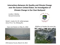
Quality and Climate Change over the Eastern United States An Investigation of Climate Change in Our Own Backyard Loretta J Mickley Harvard University Wildfires in Quebec the same day ID: 758093
Download Presentation The PPT/PDF document "Interactions Between Air" is the property of its rightful owner. Permission is granted to download and print the materials on this web site for personal, non-commercial use only, and to display it on your personal computer provided you do not modify the materials and that you retain all copyright notices contained in the materials. By downloading content from our website, you accept the terms of this agreement.
Slide1
Interactions Between Air Quality and Climate Change over the Eastern United States: An Investigation of Climate Change in Our Own Backyard
Loretta J. MickleyHarvard University
Wildfires in
Quebec the same day.
Haze over Boston on
May 31, 2010
Daniel J.
Jacob, Eric M.
Leibensperger, Amos P.K.A. Tai, Shiliang Wu
EPA Science Forum, March 14, 2012
1Slide2
2
Our work focuses on interactions of short-lived gases and particles in the atmosphere and climate change.Lifetimes in atmospheric chemistry
Centuries: SF6, some CFCs Decades:
many greenhouse gases: CO2, N2O, . . . 9-10 years: CH
4 (methane, precursor to ozone and greenhouse gas)Days-weeks: O3 (ozone), particulate matter (PM)Seconds: OH, NO
Pollution over Hong Kong
Air pollution over Hong Kong reached dangerous levels one of every eight days in 2009Slide3
Air pollution in the United States: Ozone
and fine particulate matter (PM2.5) are the two main pollutants
75 ppb (8-h average)
15
m
g m-3
(1-y av.)
Ozone
PM
2.5
Counties violating the EPA standards
3
Millions of people living in areas in violation of the standards.Slide4
The greenhouse effect keeps the Earth warm.
IPCC, 2007
Greenhouse Effect
Radiation from the earth’s surface is absorbed and re-emitted by clouds and greenhouse gases: CO
2. . .This process warms the earth.
CO
2
CO2
CO24
Change in CO
2
since mid-1800s: 280 ppm to 390 ppm.Slide5
Observed trends in surface temperature, 1880-2011.
NASA
Goddard Institute for Space Studies
Global mean temperature increase is ~0.5
oC since 1950s.
Boston/ Logan Airport
Over Boston, we see lots of year-to-year variability, but a significant trend towards warming.
Record annual mean temperature
5Slide6
Climate models show that observed global warming trends cannot be explained without human influence.
IPCC, 2007
Models with human activity.
Models with just natural processes
Observed trend
Observed trend
6Slide7
7
Basic working of climate modelsAll climate models depend on
basic physics to describe motions and thermodynamics of the atmosphere:
E.g., vertical structure of pressure is described by hydrostatic equation
Climate models also depend on
parameterizations
for many processes.
E.g., microphysics of cloud droplet formation, vegetation processes.
Tilt of earth, geography, greenhouse gas content
Weather + Climate
Input
Physics + Parameterized processes
Climate model
OutputSlide8
Simulations of future climate depend on the path of socio-economic development.
Different scenarios follow different socio-economic paths for developed and developing countries
.
IPCC 2007
Global mean surface temperature anomalies
A2 = heavy fossil fuel
B1 = alternative fuels
A1B = mix of fossil + alternative fuels
8Slide9
What do climate models
predict for future (2100) climate?Christensen et al., 2007
Annual mean Winter Summer
Temperature increases everywhere,
especially at high latitudes.
Precipitation will likely increase over high latitudes but decrease over low latitudes.
In between, the trend is not clear!
Much uncertainty in future precipitation.
Precipitation changes are more complicated.
9Slide10
How do particles affect regional climate?10Slide11
Particles affect solar radiation directly…and also indirectly by modifying cloud properties.
Pollution off U.S. east coast
Black carbon
California fire plumes
Aircraft contrails and cirrus over Europe
Light-colored particles reflect sunlight and cool the earth’s surface.
cooler
11Slide12
Comparison to observed sulfate concentrations shows good agreement.
Sequence shows increasing sulfate from 1950-1980, followed by a decline in recent years. Most of aerosol has already cleared by 2010.
1950
1960
1970
1980
1990
2001
Leibensperger
et al., 2011
Calculated trend in surface sulfate concentrations, 1950- 2001.
Clearing trend
in
particles
over United States
since 1980s suggests possible recent warming.
12Slide13
Observed US surface temperature trendGISTEMP [2010]
Is the U.S. “warming hole” a signature of cooling due to particles?
Change in temperatures over 60 year period, 1930-1990
No trend between 1930 and 1980
Warming trend after 1980
Contiguous US
o
C
13Slide14
We can examine the influence of particles on regional climate using a climate model. Most of the warming from reducing particle sources has already been realized.
Observations
Model without US particles
Standard model
US manmade particles can explain the “warming hole.”
Warming since 1990s can be attributed to reductions in particle sources.
Leibensperger
et al., 2012
Eastern US
14Slide15
How does climate change affect smog episodes?15Slide16
EPA
Roles of ozone (O3) in the atmosphere.
O
2
O3
16Slide17
Weather plays a large role in ozone air quality.
1988, hottest on record
Days
Number of summer days with ozone
exceedances
, mean over sites in Northeast
Lin et al., 2001
A very hot summer can mean more ozone
exceedances
, even if emissions of ozone precursors are declining.
17Slide18
In the Northeast, cold fronts sweep out pollution.
During heat wave:
Clear skiesFaster chemical reactionsGreater biogenic emissions
Little ventilation of pollutants
Leibensperger et al., 2008
Can climate change affect the frequency of cold fronts?
Fewer cold fronts could mean more persistent smog episodes.
18Slide19
The number of cold fronts coming through the Northeast has already showed a signal of decline.
Trend in
low-pressure systems and associated cold fronts is linked to rapid warming at high latitudes.
What does this trend mean for ozone pollution in US?Emissions of ozone precursors have declined during this period.
Mickley et al., 2004;
Leibensperger
et al., 2008
Trend
in summer low-pressure systems in S. Canada
0.14
/year
0.16
/year
observations
with increasing GHGs
with constant GHGs
model
model
19Slide20
Trend in emissions and trend in cold fronts have competing effects on surface ozone.Emissions
Ozone Episodes
Cold fronts per summer
Ozone Episodes
More heat waves, less ventilation, more persistent smog.
Smog over Baltimore in 2002.
20Slide21
Observed trends of ozone pollution and cold fronts in Northeast US
Ozone exceedance days in Northeast dropped from 30 in 1980 to 10 in 2006, but would have dropped to ≈ zero in the absence of cold-front trend.
Leibensperger
et al. [2008]
Number of ozone
episode days (O
3> 80 ppb) + Number of cold fronts, 1980-2006
Cold fronts each summer
Ozone episodes
Ozone episodes, constant climate
21Slide22
Change in
max daily 8-hour average JJA surface ozone in 2050s, relative to present-day.
Most models agree that surface ozone will increase over the
Northeast in a warming climate.
Climate penalty for air quality
:
Harvard model shows
3-7 ppb
increase in surface ozone in Midwest US in 2050s climate.
During heatwaves
, increases in ozone reach 10 ppb in future climate.
ppb
Wu et al., 2008
22Slide23
Take home messages:Reductions in particles (PM2.5) over the Eastern US has likely contributed to rapid warming
in recent years.Smog episodes in the East are sensitive to many meteorological variables, especially the frequency of cold fronts. The climate penalty:
climate change will likely worsen ozone air quality over the East.
Contiguous US
o C
Rapid warming after 1980
Acknowledgments:
23Slide24
24Slide25
25Slide26
26
O
3
O
2
h
n
O
3
Deposition
STRATOSPHERE
TROPOSPHERE
8-18 km
Lifecycle of tropospheric ozone:
production is via
oxidation of CO, VOCs, and methane in the presence of NOx.
NOx
Nonmethane volatile organic compounds (VOCs)
NOx = NO + NO
2
Human activity
Fires
Biosphere
emissions
Many processes affected by climate
NOx
NOx
NOx
VOCs
NOx
NOx
VOCs
VOCs
VOCs
VOCs
CO
CO
CH
4
CH
4
Soup of chemical reactions
Ozone is produced in the atmosphere in sunlight.
26Slide27
27
Life cycle of particulate matter (PM, aerosols)
nucleation
coagulation
condensation
wildfires
combustion
soil dust
sea salt
.
.
.
.
.
.
cycling
ultra-fine
(<0.01
m
m)
fine
(0.01-1
m
m)
cloud
(1-100
m
m)
combustion
volcanoes
agriculture
biosphere
coarse
(1-10
m
m)
scavenging
precursor gases
Climate change affects many processes, including gas-particle partitioning.
Soup of chemical reactions
NOx
NOx
NOx
NOx
NOx
VOCs
VOCs
VOCs
VOCs
VOCs
SO
2
NH
3
SO
2Slide28
Current standard (75 ppb)
EPA-recommended range for revision of standard (60-70 ppb)
Exceedances
of the ozone air quality standard
28