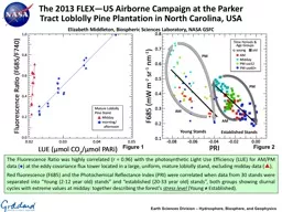
The Fluorescence Ratio was highly correlated (r = 0.96) with the photosynthetic Light - PowerPoint Presentation

The Fluorescence Ratio was highly correlated (r = 0.96) with the photosynthetic Light Use Efficiency (LUE) for AM/PM data (●) at the eddy covariance flux tower located in a large, uniform, mature loblolly stand, excluding midday data (▲). Red fluorescence (F685) and the Photochemical Reflectance Index (PRI) were correlated when data from 30 stands were separated into “Young (2-12 year old) stands” and “established (20-33 year old) stands”, both groups showing diurnal cycles with extreme values at midday: together describing the forest’s stress level (Young ≠ Established). The 2013 FLEX—US Airborne Campaign at the Parker Tract Loblolly Pine Plantation in North Carolina, USAElizabeth Middleton, Biospheric Sciences Laboratory, NASA GSFC Young Stands Established Stands Figure 1 Figure 2 Earth Sciences Division – Hydrosphere, Biosphere, and Geophysics

Name: Elizabeth M. Middleton, Biospheric Sciences, NASA GSFC E-mail: elizabeth.m.middleton@nasa.gov Phone: 301-614-6670 References: Middleton, E.M., U. Rascher, L.A. Corp, K.F. Huemmrich, B.D. Cook, A. Noormets, A. Schickling , F. Pinto, L. Alonso, A. Damm, L. Guanter, R. Colombo, P.K.E. Campbell, D.R. Landis, Qingyuan Zhang, M. Rossini, D. Schuettemeyer, and R. Bianchi (2017). The 2013 FLEX—US Airborne Campaign at the Parker Tract Loblolly Pine Plantation in North Carolina, USA. Remote Sensing, Special Issue Remote Sensing of Vegetation Fluorescence and Photosynthetic Efficiency, June 2017. http:// www.mdpi.com/2072-4292/9/6/612/pdf Technical Description of Images: Data were collected at the managed Parker Tract Loblolly Pine forest located near Plymouth, North Carolina, having multiple stands of varying age. The data were obtained with the HyPlant airborne system (PI: U. Rascher, Jülich Forschungszentrum): Fluorescence was derived from high spectral resolution measurements (≤ 0.3 nm) acquired with HyPlant’s FLUO module, whereas hyperspectral reflectance measurements (≤ 5 nm) were made with HyPlant’s DUAL spectrometer module. Stand heights and uniformity were confirmed using LiDAR data acquired simultaneously with the co-manifested G-LiHT airborne package (GSFC). Figure 1: Fluxes at the eddy covariance tower (NC2) located in one of the mature Loblolly Pine stands (age class 4, 27–33 year) : the Fratio (F685/F740) vs. the photosynthetic Light Use Efficiency (LUE, GPP/APARestimated, J µmol−1 PAR sr−1 nm−1) for two time groups, mid-day (red triangles) and morning/afternoon combined (blue circles). The relationships are linear but depend on time of day (r2 = 0.84, p ≤ 0.000, F-ratio = 32.02, n = 31; p ≤ 0.000). Stronger results were obtained for the combined morning/afternoon observations only (and leaving out the mid-day), LUE (r = 0.96, SEM of 0.002), where, LUE = 0.016 + 0.027 x Fratio. Note: Midday observations are not useful for relating the Fluorescence Ratio to tower LUE.Figure 2: Hysteresis is described by combining the red fluorescence (F685) with the Photochemical Reflectance Index (PRI) acquired at four times over the diurnal cycle at 30 Loblolly Pine stands of varying stand ages, by combining responses of F685 and the PRI: all ROI stands, including the NC2 tower stand. The PRI is a normalized difference reflectance index using green spectral bands [PRI = (R530 – R570)/(R530 + R570)], where the R530 is the physiologically active wavelength.Key: (A) The tower flux data and airborne fluorescence data are separated into two temporal groups: midday (▲) and combined morning and afternoon (●). (B) Four times of day are shown for both young and established Loblolly Pine stands, where the arrows indicate the opposite direction of changing values in the morning and the afternoon. Scientific Significance: Together the red and far-red fluorescence (F685, F740) expressed as the Fratio were capable of describing tower LUE, except at midday when both GPP and incoming PAR were maximal. Both the PRI and F685 were necessary to describe forest stress over the diurnal cycle, and to distinguish young from mature stands. Earth Sciences Division – Hydrosphere, Biosphere, and Geophysics

Near Real-Time Flood Detection and Socioeconomic Impact Assessment in the Lower Mekong River Basin John Bolten1, Perry Oddo1,2, Aakash Ahamed3 1Hydrological Sciences Lab, NASA GSFC; 2USRA ; 3Stanford University, Geophysics Figure 1 Earth Sciences Division – Hydrosphere, Biosphere, and Geophysics MODIS-derived surface water extents are used to produce flood depth estimates in near real-time. Flood depth estimates are then fed into a standardized flood damage framework to produce damage estimates based on inundated land cover and affected infrastructure. The rapid initial estimates of socioeconomic impacts can provide valuable information to governments, international agencies, and disaster responders in the wake of extreme flood events.DescriptionArea (km2) Damages (USD) Rice - 1 crop/yr 12,192.01 2,317,168 Mixed Annual Crops 1,425.17 1,435,970 Cleared before 2010 35.36 35,661 Orchard 242.66 73,169 Flooded Forest 3,113.91 28,265,720 Grassland/Sparse Vegetation1,767.45 497,578 Deciduous Shrubland1,155.41 319,502 Urban205.91 12,604 Barren - Rock Outcrops67.85 - Industrial Plantation1.30 355 Deciduous Broadleaved7.15 56,089 Evergreen/ Broadleaved2.18 17,931 Forest Plantation0.00 - Bamboo Scrub/Forest11.09 101,454 Coniferous Forest 0.00 - Mangrove 1.71 10,693 Marsh/Swamp 493.05 151,308 Aquaculture 5.99 2,496 Aquaculture Rotated with Rice 17.56 3,316 (B) (C) (D) Damages (USD / m 2 ) (A) Table 1

Earth Sciences Division – Hydrosphere, Biosphere, and Geophysics Name: John Bolten, Hydrological Sciences Lab, NASA GSFC E-mail: john.bolten@nasa.gov Phone: 301-614-6529 References:Fayne, J. V. et al. Flood mapping in the lower Mekong River Basin using daily MODIS observations. International Journal of Remote Sensing 38, 1737–1757 (2017).Ahamed, A. & Bolten, J. D. A MODIS-based automated flood monitoring system for southeast asia. International Journal of Applied Earth Observation and Geoinformation 61, 104–117 (2017). Cham, T. C., Mitani, Y., Fujii, K. & Ikemi, H. Evaluation of flood volume and inundation depth by GIS midstream of Chao Phraya River Basin, Thailand. in WIT Transactions on The Built Environment (ed. Brebbia , C. A.) 1, 1049–1060 (WIT Press, 2015). Ahamed, A., Bolten, J., Doyle, C. & Fayne, J. Near Real-Time Flood Monitoring and Impact Assessment Systems. in Remote Sensing of Hydrological Extremes (ed. Lakshmi, V.) 105–118 (Springer International Publishing, 2017). doi:10.1007/978-3-319-43744-6_6Kok, M., Huizinga, H. J., Vrouwenfelder , A. & Barendregt, A. Standard method 2004. Damage and casualties caused by flooding. (Rijkswaterstaat, 2004).Leenders, J. K., Wagemaker, J., Roelevink, A., Rientjes, T. H. M. & Parodi, G. Development of a damage and casualties tool for river floods in northern Thailand. in Flood Risk management: Research and Practice 1707–1715 (Taylor & Francis, 2009).Data Sources: Optical and near infrared bands from MODIS products (MOD09Q1; MOD09GQ; MOD35) to detect surface water extent. Land cover data for Mekong region was produced by project partners at the Mekong River Commission. Socioeconomic data for impact analysis obtained from NASA Socioeconomics Data and Applications Center (SEDAC) and OpenStreetMap. Case study example (pictured) uses flood extent map from ESA Advanced Synthetic Aperture Radar, Wide Swath Mode.Technical Description of Figures:Figure 1: (A) Flood extent with interpolated triangular irregular network (TIN); (B) Flood depth raster produced by merging interpolated water surface and underlying DEM; (C) Land cover map for Lower Mekong Basin; (D) Socioeconomic Damage estimates from impact assessment.Table I: Economic damage estimates for each land cover type. Estimates produced using depth-damage functions and estimated flood depths (Kok et al. 2004) Scientific significance, societal relevance, and relationships to future missions: Flood damage assessments are frequently used to quantify the economic losses in the wake of storms. These assessments are critical for understanding the effects of flooding on the local population, and for informing decision-makers about future risks. Remote sensing systems provide a valuable tool for monitoring flood conditions and assessing their severity more rapidly than traditional post-event evaluations. Improved land cover and flood depth assessments result in a more refined understanding of losses throughout the Mekong River Basin. Data from VIIRS and radar imagery from Sentinel I could be used to improve flood detection capabilities in future studies.

Airborne LUnar Spectral Irradiance (air-LUSI) Mission Design Kevin R. Turpie 1,5 , Steve Brown 2, John Woodward2, Andrew Gadsden3, Tom Stone4 1University of Maryland, Baltimore County, 2National Institute of Standards and Technology, 3 University of Guelph, 4 U.S. Geological Survey, 5Ocean Ecology, NASA GSFC a ir-LUSI telescope and autonomous, robotic mount is designed to acquire unprecedentedly accurate measurements of lunar spectral irradiance from an ER-2 aircraft flying at 21km altitude. Earth Sciences Division – Hydrosphere, Biosphere, and GeophysicsFigure 1Figure 3Figure 2

Name: Kevin Turpie, Ocean Ecology, NASA GSFC, UMBC E-mail: Kevin.R.Turpie@nasa.gov Phone: 301-286-9996 References: Turpie, K.R., Eplee, R.E., Meister, G., “Propagation of Visible Infrared Imaging Radiometer Suite (VIIRS) calibration uncertainty trends to ocean color data,” Proceedings of the SPIE 9111, Ocean Sensing and Monitoring XX , 9607-60 (Aug 12, 2015).Cramer, C. E., et al., "Precise measurement of Lunar spectral irradiance at visible wavelengths", Journal of Research of the National Institute of Standards and Technology. 118, 396-402 (2013). Kieffer, H. H. and T. C. Stone, “The Spectral Irradiance of the Moon, " Astronomical Journal 129, 2887-2901 (2005). Data Sources: ROLO model, EOS, NPP, JPSS, SeaWiFS, CNES Pleiades, SOURCE, SAO, OMI.Technical Description of Figures:Figure 1: Concept drawing of the Irradiance Instrument Subsystem (IRIS) combined with the Autonomous Robotic Telescope Mount Instrument Subsystem (ARTEMIS), which keeps the instrument fixed on the Moon. Figure 2: The air-LUSI system is situated in the wing pod of the ER-2 high altitude aircraft. Figure 3: Lunar spectral irradiance measured at two different phases from the original LUSI system from Mt. Hopkin in Arizona. Scientific significance, societal relevance, and relationships to future missions: The airborne LUnar Spectral Irradiance (air-LUSI) mission will measure lunar spectral irradiance with unprecedented accuracy from a high-altitude aircraft (ER-2). This careful characterizing will make the Moon a stable and consistent extra-terrestrial calibration reference for Earth observing satellites. This will be especially beneficial to calibration-sensitive ocean color missions, such as the upcoming PACE and JPSS (VIIRS) missions, and retrospectively for the SeaWiFS, EOS (MODIS), and S-NPP (VIIRS) data records. Earth Sciences Division – Hydrosphere, Biosphere, and Geophysics

Impact of New Reference Frame, ITRF2014, on Rate of Change of Global Mean Sea LevelF.G. Lemoine1 , N.P. Zelensky2, B.D. Beckley 2, D.S. Chinn2 , & D.E. Pavlis2 1Geodesy and Geophysics Laboratory, NASA GSFC , 2SGT Inc. Radial Orbit Drift based on Satellite Laser Ranging (SLR) and DORIS Doppler data from 1992 to 2016 for TOPEX/Poseidon, Jason-1, Jason-2 & Jason-3, illustrating the impact on the Global Mean Sea Level (GMSL) rate of using the new realization of the International Terrestrial Reference Frame (ITRF), ITRF2014, compared to ITRF2008. We use an observation geometry for an ocean radar satellite altimeter showing satellite tracking systems (SLR, DORIS, GPS). Earth Sciences Division – Hydrosphere, Biosphere, and Geophysics TOPEX: 1992-2002 Jason-1,2,3: 2002-2017 Longitude ( deg )Latitude (deg.)ALTIMETER SATELLITE MEASUREMENT SYSTEMFigure 1Figure 2

Name: FrankG. Lemoine, NASA GSFC, Geodesy & Geophysics Laboratory Code 61A E-mail: Frank.G.Lemoine@nasa.gov Phone: 301-614-6109 References:Zelensky, N.P.. , F.G. Lemoine, B.D. Beckley, D.S. Chinn and D.E. Pavlis (2017), “Impact of ITRF 2014 realizations on altimeter satellite precise orbit determination” Adv. Space Res., doi:10.1016/j.asr.2017.07.044.Lemoine, F.G ., D.S. Chinn, N.P. Zelensky, J.W. Beall, K. Le Bail (2016), “The development of the GSFC DORIS Contribution to ITRF2014,” Adv. Space Res., 58(12), 2520–2504, doi:10.1016/j.asr.2015.12.043.Beckley B. D., F.G. Lemoine, S. B. Luthcke, R. D. Ray, N. P. Zelensky (2007), “A reassessment of global and regional mean sea level trends from TOPEX and Jason-1 altimetry based on revised reference frame and orbits”, Geophys. Res. Lett., 34(14), L14608. Data Sources: (1) Sea surface heights (SSH) are derived from reprocessed TOPEX/Poseidon, Jason-1, 2, & 3 radar altimeter data via the NASA MEaSUREs Integrated Multi-Mission Ocean Altimeter Data for Climate Research (http://dx.doi.org/10.5067/ALTTS- TJ124 ); (2) Satellite Laser Ranging (SLR) tracking data provided by the International Laser Ranging Service (ILRS), (http://ilrs.gsfc.nasa.gov;) (3) DORIS satellite tracking data provided by the International DORIS Service (IDS), (http://ids-doris.org); (4) Reference frame realizations, including ITRF2014 and ITRF2008, provided by the International Earth Rotation and Reference Systems (IERS), (http://www.iers.org/).Technical Description of Figure: Figure 1: A precise geodetic reference frame and precise orbits are a fundamental requirement for satellite altimetry. The terrestrial reference frame is the means by which the orbit reference is computed for the analysis of satellite altimeter data. Error in the terrestrial coordinates for the tracking stations, and in the frame will transfer to the orbit and through the orbit to the altimeter measurements. Figure 2: In Zelensky et al. (2017) we evaluated the impact on the global rate in mean sea level of the update in the reference frame realization from ITRF2008 to ITRF2014, recently released. Reference frame realizations are updated every 5-6 years as new stations are added and old tracking stations disappear and as geophysical models are improved. The change in sea level rate due to the intrinsic errors in the reference frame is a factor in the total sea level error budget. In this figure we show the impact of adopting ITRF2014 compared to the now-out-of-date realization, ITRF2008, made available in 2009. While now we see changes of ±0.3 mm/yr in GMSL, in 2007 due to the switch to ITRF2005 we saw changes in GMSL up to ±1.5 mm/yr at the high latitudes (Beckley et al., 2007).Scientific significance, societal relevance, and relationships to future missions: The terrestrial reference frame is the foundation of virtually all space-based, airborne, and ground-based Earth observations. Positions of objects and data measurements are determined within an underlying TRF and the accuracy with which objects can be positioned ultimately depends on the stability and quality of the underlying frame. The TRF makes it possible to intercompare and interrelate observations in space and time. Altimeter missions measuring ocean surface topography (TOPEX/Poseidon, Jason-1, Jason-2, Jason-3, Sentinel-3A, Jason-CS, SWOT) or cryosphere change (ICESAT, ICESAT-2, Cryosat-2) situate (geolocate) their data in a reference frame that is defined by the underlying orbits computed for these satellites based on geodetic tracking data (Satellite Laser Ranging, DORIS Doppler, Global Navigation Satellite Systems, GNSS). The accuracy of a TRF realization depends on the quantity, distribution, and accuracy of the geodetic data used to determine the coordinates (position & velocity) of the reference points. A TRF realization is always better determined over the time span of the data it incorporates, and degrades in extrapolation. TRF realizations are periodically recomputed to include new data, and take into account improvements in background modeling. Earth Sciences Division – Hydrosphere, Biosphere, and Geophysics