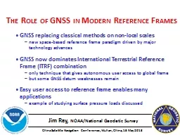
The Role of GNSS in Modern Reference Frames GNSS replacing classical methods on nonlocal scales new spacebased reference frame paradigm driven by major technology advances ID: 904575
Download The PPT/PDF document "Jim Ray, NOAA/National Geodetic Survey" is the property of its rightful owner. Permission is granted to download and print the materials on this web site for personal, non-commercial use only, and to display it on your personal computer provided you do not modify the materials and that you retain all copyright notices contained in the materials. By downloading content from our website, you accept the terms of this agreement.
Slide1
Jim Ray, NOAA/National Geodetic Survey
The Role of GNSS in Modern Reference Frames
GNSS replacing classical methods on non-local scales new space-based reference frame paradigm driven by major technology advances GNSS now dominates International Terrestrial Reference Frame (ITRF) combination only technique that gives autonomous user access to global frame but some GNSS datum weaknesses remain Easy user access to reference frame enables many applications example of studying surface pressure loads discussed
China Satellite Navigation Conference, Wuhan, China, 15 May 2013
Slide2Since ancient times, positions measured with respect to nearby visible points
angles
& distances allow triangulation & trilateration of small networksspirit leveling used for relative heightssimultaneous adjustment of redundant observations gave rise to Gauss’ least-squares methodaccuracies can attain <~1 mm over <~1 km distances
Horizontal & vertical components normally treated separatelydriven by measurement technologies & by applicationshorizontal control for property bounds
vertical control for gravity variations &
water flow
Classical Terrestrial Surveys
02
Slide3Classical Survey Components
03
Control MarkControl MarkSurvey Network(inter-visible stations)
Theodolites & Total StationsAngle, Distance &
Height Measurements
Slide4For larger regional/national reference frames
must aggregate many local survey networks
not always well connected to each other (especially across oceans)gives rise to network distortions, inhomogeneous coverage, & variable accuracieslocal survey errors accumulate over distanceframes not consistent between different authoritiesInternational standards began in 1875
Metre Convention led to SI physical units1884 Conference led to Greenwich prime meridian for longitudes
but accurate geocentric
global frame not possible
till nearly 100
yr later
Extension to National Reference Frames
04
Main Triangulation (Horizontal) Networks
(early 1980s)
Slide5
Era of space geodesy
! New Geodetic Paradigm: Technological ElementsNew, high-accuracy techniques enabled on global scale: Digital electronics & computers: fast switches broadband sampling massive data storage cross-correlators efficient data analysisAtomic clocks: coherent obs >1 s accurate short-interval timing remote synchronization simplified modelingArtificial satellites: continental scale inter-visibility geocenter sensitivity forced international
cooperation for global tracking interferometry phase tracking at cm → dm wavelengths precise unambiguous group delays wide station separation measure accurate geopotential allow GNSS positioning anywhere, anytime eliminate dependence
on dense ground nets absolute geocentric positions
inter-station clock offsets
estimated in data analysis
global timekeeping <~1 µs
accurate data time tags Kepler’s 3rd law constrains
satellite radial dynamics
05
Slide6Key inventions & early technology development ~1950s
Practical implementation
phase 1960s → 1970sSatellite Laser Ranging (SLR)TRANSIT Doppler
Very Long Baseline (Radio) Interferometry (VLBI)
Brief History of Space Geodetic Techniques (1/3)
06
Slide7Maturation phase
1980s → 1990s
Doppler Orbitography & Radiopositioning by Satellite (DORIS)Global Navigation Satellite Systems (GNSS): · GPS
· GLONASS
Brief History of Space Geodetic Techniques (2/3)
07
Slide8Expansion & exploitation phase
1990s/2000s →
new GNSS: · BEIDOU · GALILEO · Regional augmentationsroutine national & international services established (e.g., IGS)many scientific/geophysical networks installed
Brief History of Space Geodetic Techniques (3/3)
08
Global Reference
Network of
International GNSS
Service (IGS)
GEONET displacements after
11 Mar 2011 Tohoku earthquake
Plate Boundary
Observatory (PBO)
in western USA
Slide9relatively low user costs (not including GNSS itself)
service available for anybody, anywhere, anytime
user can operate autonomouslyinherently designed for real-time operationslow-accuracy mode via GNSS broadcast open servicehigh-accuracy mode via augmentation services (e.g., IGS)user positions reach ~1 cm accuracy in post-processing mode (24 hr data)real-time positions reach ~1 dm level (absolute geocentric mode)differential positions attain sub-cm precision over regional scalesGNSS networks can serve many objectives simultaneously, e.g.:
geodynamics, water vapor sensing, ionosphere monitoring, geodetic/survey referencing, time transfer, land cover probe, . . .
Unique Advantages of GNSS
09
Slide10GPS frame dominates
International Terrestrial Reference Frame
latest ITRF realization is 2008GPS co-locations link all techniquesGPS is 60% of all ITRF stations (560 out of 934)GPS results very homogeneous & stable in timeWRMS accuracy of weekly points: dN, dE ~ 1.5 mm; dU ~ 4.5 mm
But GNSS weaknesses remainGNSS cannot observe geocenter accurately due to parameter correlations → so ITRF origin based on SLR
(stable at ~0.5 mm/yr)
GNSS frame scale fixed to ITRF scale to estimate satellite antenna offsets
→ so
ITRF scale based on SLR +
VLBI (stable at ~0.2 mm/yr
)
GNSS position time series have many breaks due to
equipment
changes
draconitic
harmonics abound due to orbit-related
mismodeling
GNSS Contributions to ITRF
10
[Z.
Altamimi
et al., 2011]
Station Position WRMS
Slide11GPS dominates daily
Polar Motion
results since mid-1990sdue to robust global tracking networkWRMS daily accuracy: ~ 30 µasequals ~1 mm global shift at Earth’s surfaceBut systematic errors remain significant
errors in international model for EOP 12h & 24h tidal variations → errors alias into orbital & other parametersmismodeling of orbital dynamics (empirical solar radiation pressure) → propagates draconitic signals & harmonics
mishandling of frame rotational stability by Analysis Centers
non-linear motions at most GNSS stations
possible instabilities in ITRF realization
Length-of-day (LOD) also measured
(but
not UT1 or
nutations
)
GNSS Contributions to Earth Orientation
11
[Z.
Altamimi
et al., 2011]
Polar Motion
x,y
Residuals
PMx
: VLBI SLR GPS DORIS
PMy
: VLBI SLR GPS DORIS
Slide12GNSS User Access to ITRF
12
IGS Reference Network in ITRFIGS tracks GNSS globally: reference frame of ITRF ground stations transferred to satellite positions & clocksUser tracks GNSS locally: reference frame transferred to user position
Positioning in ITRF using GNSSPrecise Differential Positioning user + other nearby GNSS data + precise GNSS orbits (IGS)→ user relative location
Absolute Positioning (PPP) user data
+ precise GNSS orbits &
clocks
(IGS)→ user geocentric (ITRF) location
Two approaches used for frame transfer:
Merits of Two GNSS Positioning Approaches
13
Precise Differential Positioning data analysis is easier due to common mode error rejection very precise relative positions few mm precision, depending on distance of reference stations easier to implement in real-time over regional/local scales infrastructure requirements adjustable to user application user accuracy depends on errors in reference positions & data best performance requires dense ground networks not practical over global scales many operations are private major global infrastructure required, both ground network & data analysis user data analysis must be highly consistent with models used to make global orbit & clock products
Disadvantages:
Advantages:
Absolute Positioning (PPP)
autonomy of operation
works for anybody, anywhere,
anytime
absolute geocentric positions
daily accuracies: ~4-5 mm N,E
~10 mm U
Slide14Surface mass
load displacement time series
for all GPS stations6-hr NCEP atmosphere model12-hr ECCO non-tidal ocean modelmonthly GLDAS surface ice/water, cubic detrended to remove model driftall computed for center-of-frame (CF) originsum is linearly detrended & averaged to middle of each GPS weekload model data from 1998.0 to 2011.0 [courtesy of T. van Dam]GPS
station position time series from 1st IGS reprocessinganalysis generally consistent with IERS 2010 Conventionscombined results from up to 11 Analysis Centers706 globally distributed stations, each with >100 weeks
data from 1998.00 to 2011.29
Helmert
alignment (no scale)
w.r.t
. cumulative solution uses a well-distributed subnetwork to minimize aliasing of local load signals
care taken to find position/velocity
discontinuities
Study
dN
,
dE
,
dU
non-linear residuals (1998.0 – 2011.0)
bias errors not considered here !
Example
of Crustal Loading Studied with
GNSS
14
Slide15Load models most effective in
height for GLSV (Kiev)
reduce dU scatter by 51%reduce annual dU amplitude by 73% model not effective for dN, dEinland continental siterelatively large atmosphere pressure variations
GPS Position Time Series – “Best” Load Fit15
GLSV (Kiev)
Slide16Load models least effective in
height for PARC (S. Chile)
increase dU scatter by 15%reduce annual dU amplitude by 38% model not effective for dN, dEcoastal siteatmosphere pressure effects damped by nearby oceans
GPS Position Time Series – “Worst” Load Fit16PARC (S. Chile)
Slide17GPS Stations With Smallest Height Scatter
17
LAGO (coast)GLPS (island)dN & dE scatters (~1 mm) are not the “best” . . .dU scatters have same WRMS but different characters
possibly related to weaknesses of IB assumption or load models
Slide18(GPS – Load) Comparison Statistics (706 stations)
18
WRMS Changesmedian GPS WRMS (mm)median Load RMS (mm)median(GPS – Load) WRMS (mm)median WRMS reduction (%)% of stations with lower WRMSdN1.40.51.33.872.0dE1.450.4
1.41.662.9dU4.62.63.8
15.2
87.4
Annual Amplitude Changes
median GPS annual (mm)
median Load annual (mm)
median
(GPS – Load) annual (mm)
median annual (
corr
/no
corr
) ratio
% of stations with lower annual amp
dN
0.9
0.45
0.65
0.8
70.7
dE
0.8
0.4
0.7
0.9
59.3
dU
3.6
2.4
1.7
0.5
87.1
Load corrections are effective to reduce WRMS & annual amps
for most stations,
esp
for
dU
– but less for
dN
& even less for
dE
Slide19(GPS – Load) Comparison Statistics (706 stations)
19
WRMS Changesmedian GPS WRMS (mm)median Load RMS (mm)median(GPS – Load) WRMS (mm)median WRMS reduction (%)% of stations with lower WRMSdN1.40.51.33.872.0dE1.450.4
1.41.662.9dU4.62.63.8
15.2
87.4
Annual Amplitude Changes
median GPS annual (mm)
median Load annual (mm)
median
(GPS – Load) annual (mm)
median annual (
corr
/no
corr
) ratio
% of stations with lower annual amp
dN
0.9
0.45
0.65
0.8
70.7
dE
0.8
0.4
0.7
0.9
59.3
dU
3.6
2.4
1.7
0.5
87.1
Load corrections are effective to reduce WRMS & annual amp
But most residual variation remains,
esp
in
dN
&
dE
Slide20IGS Results – dN With/Without Loads
20
dN load corrections have no impact on noise floor assessmentlocal site & non-load errors overwhelmingly dominateA2 : 0.5 0.6Error Model: WRMS2 =
WRMSo2 + (Ai * AnnAmpi)2 + WRMSi2
WRMS
o
2
= noise floor
Slide21IGS Results – dE With/Without Loads
21
dE load corrections have no impact on noise floor assessmentlocal site & non-load errors overwhelmingly dominateA2 : 0.5 0.6Error Model: WRMS2 =
WRMSo2 + (Ai * AnnAmpi)2 + WRMSi2
WRMS
o
2
= noise floor
Slide22IGS Results – dU With/Without Loads
22
dU load corrections move results much closer to noise floorbut local site & non-load errors still dominateA2 : 0.5 0.6
Slide23IGS Results – dU With/Without Loads
23
A2 : 0.5 0.6“Best” 2 stations in dU (WRMS = 2.2 mm) are:LAGO (S. coast, Portugal) & GLPS (island, Pacific Ocean)GLPSLAGO
Error Model: WRMS2 = WRMSo2
+
(A
i * AnnAmpi
)2
+ WRMS
i
2
WRMS
o
2
= noise floor
Slide24Decomposition of Weekly GPS Position Errors
24
IGS Error Budget for Weekly IntegrationsWRMSo (mm)median Annual Amps (mm)median site WRMSi (mm)median total WRMS(mm)thermal(via pairs)models + analysistotalloadstotal
dN0.40.50.650.450.91.01.4
dE0.4
0.6
0.7
0.4
0.8
1.1
1.45
dU
1.3
1.7
2.2
2.4
3.6
2.9
4.6
Infer site
WRMS
i
2
using:
WRMS
o
2
+ (A *
AnnAmp
i
)
2
+ WRMS
i
2
= WRMS
2
where A
2
= 0.6
Noise
floor
WRMS
o
& local site
errors
WRMS
i
dominate
over
loads
esp
for N & E components
Non-
load
GPS
annual
errors
are as large as
annual
load
signals
unless load models missing ~half of total signal
Slide25Load corrections reduce WRMS & annual amps for most stations
but most residual variation remains,
esp for dN & dEimplies load models are inaccurate &/or other sources of scatter/errorStation weekly scatter can be decomposed into 3 categories: dN dE dU global average floor WRMSo (mm) 0.65 0.7 2.2 median annual amp WRMS (mm) 0.7 0.6 2.8 (for A
2 = 0.6; about half due to loads) median local site WRMSi (mm) 1.0 1.1 2.9 total WRMS (mm) 1.4 1.45 4.6
Harmonics of GPS draconitic
period are pervasive
strong spatial correlations imply a major orbit-related
source
but significant
draconitics
in close pair differences imply smaller local contributions likely too
1.04
cpy
signal must contribute to observed annual variations but magnitude is unknown
Major non-load technique improvements still badly needed!
Summary of Current GPS Position Errors
25
Slide26GPS
positioning accuracy now in plateau phase
future progress limited by known or suspected systematic errors : • draconitic errors related to orbit modeling • errors in IERS subdaily Earth orientation tide model • unmodeled thermal expansion of antenna structures & Earth surface • multipath errors (esp due to near-field) & antenna environment • antenna calibration errors • frequent position discontinuities (equipment changes)
New GNSS systems offer hope to reduce some current errorsdifferent constellation designs & orbital resonancessome better signal structures (more resistant to multipath)but also much greater multi-GNSS complexity (esp
inter-system biases)
Major challenges
for the future include:
understanding how best to use multi-GNSS systems together
m
uch more robust & reliable international infrastructures
(ground tracking networks & data analysis)
large reduction in station discontinuities & disruptions
secure governmental support with strong international cooperation
Prospects for Future GNSS Evolution
26
Slide27Thank You!