PPT-How are tropical cyclones represented in operational model initial conditions?

Author : celsa-spraggs | Published Date : 2019-03-03

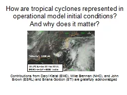
And why does it matter Gary Lackmann North Carolina State University 5 July 2012 Contributions from Daryl Kleist EMC Mike Brennan NHC and John Brown ESRL and Briana

Presentation Embed Code

<iframe width="560" height="315" src="https://www.docslides.com/embed/754917" frameborder="0" allowfullscreen></iframe>

Download Presentation

Download Presentation The PPT/PDF document "How are tropical cyclones represented in..." is the property of its rightful owner. Permission is granted to download and print the materials on this website for personal, non-commercial use only, and to display it on your personal computer provided you do not modify the materials and that you retain all copyright notices contained in the materials. By downloading content from our website, you accept the terms of this agreement.

How are tropical cyclones represented in operational model initial conditions?: Transcript

Download Document

Here is the link to download the presentation.
"How are tropical cyclones represented in operational model initial conditions?"The content belongs to its owner. You may download and print it for personal use, without modification, and keep all copyright notices. By downloading, you agree to these terms.