PPT-Probe analysis and data preprocessing

Author : cheryl-pisano | Published Date : 2016-06-01

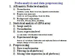
Affymetrix Probe level analysis Normalization Constant Loess Rank invariant Quantile normalization Expression measure MAS 40 LIWong dChip MAS 50 RMA Background

Presentation Embed Code

Download Presentation

Download Presentation The PPT/PDF document "Probe analysis and data preprocessing" is the property of its rightful owner. Permission is granted to download and print the materials on this website for personal, non-commercial use only, and to display it on your personal computer provided you do not modify the materials and that you retain all copyright notices contained in the materials. By downloading content from our website, you accept the terms of this agreement.

Probe analysis and data preprocessing: Transcript

Affymetrix Probe level analysis Normalization Constant Loess Rank invariant Quantile normalization Expression measure MAS 40 LIWong dChip MAS 50 RMA Background adjustment PMMM PM only RMA GCRMA. : . Coregistration. and Spatial Normalisation. Cassy . Fiford. and . Demis. Kia. Methods for Dummies 2014. With thanks to Gabriel Ziegler. 1. . Preprocessing. Recap. 2. . Coregistration. 3. Spatial Normalisation. Acquisition, preprocessing and analysis of spectra. Raman . spectrometer. . scheme. Acquisition, preprocessing and analysis of Raman spectra. 2. Credits: http://. www.doitpoms.ac.uk. /. tlplib. /. raman. Presenter: Nizar Habash. COMS E6998: Topics in Computer Science: Machine Translation. February 7, 2013. Reading Set #1. Papers Discussed. Nizar Habash and Fatiha Sadat. 2006. . Arabic Preprocessing Schemes for Statistical Machine Translation. Jiongqian. (Albert) Liang. *, David . Fuhry. *, David . Maung. *, . Alexandra . Borstad. +. , Roger . Crawfis. *, Lynne Gauthier. +. , . Arnab. Nandi*, Srinivasan Parthasarathy*. * Department of Computer Science and Engineering.. HCI571 Isabelle Bichindaritz . 1. Working with Data. Data. . Summarization. 9/28/2012. HCI571 Isabelle Bichindaritz . 2. Learning Objectives. Why do we need to preprocess data?. Descriptive data summarization. 严超赣. Chao-Gan Yan, Ph.D.. yancg@psych.ac.cn. http://. rfmri.org. /. yan. Institute of Psychology, Chinese Academy of Sciences. DPARSF. (Yan and Zang, 2010). 2. Data Processing Assistant for Resting-State fMRI (DPARSF). Ahmedul Kabir. TA, CS 548, Spring 2015. 1. Preprocessing Techniques Covered. Standardization and Normalization. Missing . value . replacement. Resampling. Discretization. Feature . Selection. Dimensionality Reduction: PCA. Learning Objectives. Be . able to describe when and why image corrections are appropriate or . necessary. Give . examples of some common approaches to image . correction. Understand the processing steps of Landsat data. Using SQL to investigate anomalies on Parker Solar Probe. David Edell <. david.edell@jhuapl.edu. >. JHU/APL. 27 November 2017. Parker Solar Probe – SpaceWire DB Analysis Tool. 1. Overview. 27 November 2017. Resting-State fMRI (. Part II). Chao-Gan YAN, Ph.D.. 严超赣. y. cg.yan@gmail.com. http://. rfmri.org. Research Scientist . The . Nathan Kline Institute for Psychiatric . Research. Research Assistant Professor . 严超赣. Chao-Gan Yan, Ph.D.. yancg@psych.ac.cn. http://. rfmri.org. /. yan. Institute of Psychology, Chinese Academy of Sciences. DPARSF. (Yan and Zang, 2010). 2. Data Processing Assistant for Resting-State fMRI (DPARSF). HCP . D. ata. Qunqun. Y. u. . Dr.. . Steve. . Marron. ,. . Dr.. . Kai. . Zhang. . &. . Dr.. . Ben. . Risk. University. . of. . North. . Carolina. . at. . Chapel. . Hill. Human. . Illumina. Array . Data. SPH 247. Statistical Analysis of. Laboratory Data. 1. May 7, 2010. SPH 247 Statistical Analysis of Laboratory Data. Basic Design of Expression Arrays. For each gene that is a target for the array, we have a known DNA sequence.. What Is Data Mining?. Many people treat data mining as a synonym for another popularly used term, knowledge discovery from data, or KDD, while others view data mining as merely an essential step in the process of knowledge discovery. .

Download Document

Here is the link to download the presentation.
"Probe analysis and data preprocessing"The content belongs to its owner. You may download and print it for personal use, without modification, and keep all copyright notices. By downloading, you agree to these terms.