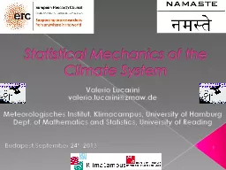
PPT-Statistical Mechanics of the Climate System PowerPoint Presentation

Valerio Lucarini valeriolucarinizmawde Meteorologisches Institut Klimacampus University of Hamburg Dept of Mathematics and Statistics University of Reading 1

Upload by cheryl-pisano
Published on 2017-04-12

Presentation Embed Code

<iframe width="560" height="315" src="https://www.docslides.com/embed/536843" frameborder="0" allowfullscreen></iframe>

Download Presentation

Download Presentation The PPT/PDF document "Statistical Mechanics of the Climate Sys..." is the property of its rightful owner. Permission is granted to download and print the materials on this web site for personal, non-commercial use only, and to display it on your personal computer provided you do not modify the materials and that you retain all copyright notices contained in the materials. By downloading content from our website, you accept the terms of this agreement.