/
A Tale of Two Careers (tightly intertwined) A Tale of Two Careers (tightly intertwined)

A Tale of Two Careers (tightly intertwined) - PowerPoint Presentation

danika-pritchard
danika-pritchard . @danika-pritchard
Follow
346 views
Uploaded On 2018-11-04

A Tale of Two Careers (tightly intertwined) - PPT Presentation

Andrew J Viterbi Presidential Chair Professor of Electrical Engineering University of Southern California September 25 2017 Careers Timeline JPLUSC 19571963 UCLA 19631975 UCSD 19751985 ID: 713002

state time discrete markov time state markov discrete noise continuous sequence gaussian error theory spread loop filter varying linear

Share:

Link:

Embed:

Download Presentation from below link

Download Presentation The PPT/PDF document "A Tale of Two Careers (tightly intertwin..." is the property of its rightful owner. Permission is granted to download and print the materials on this web site for personal, non-commercial use only, and to display it on your personal computer provided you do not modify the materials and that you retain all copyright notices contained in the materials. By downloading content from our website, you accept the terms of this agreement.


Presentation Transcript

Slide1

A Tale of Two Careers(tightly intertwined)

Andrew J. Viterbi

Presidential Chair Professor of Electrical Engineering

University of Southern California

September 25, 2017Slide2

Careers’ Timeline

JPL/USC 1957-1963

UCLA 1963-1975

UCSD 1975-1985

Linkabit

1969-1985

UCSD 1985-1994 Qualcomm 1985-2000

------------------------------------------------------------------------------

USC/Technion/UCSD 2000-- Viterbi Group 2000--Slide3

External Influences

Andrey

Andreyvich

Markov (1906)

The Cold War (1948-1989)

Digital (R)Evolution (1948---)Slide4

Andrey Andreyevich Markov (1856-1922)

Disciple of P.

Chebyshev

Markov Chains (1906)

(AKA Sequences, Processes)

Politically active in 2

nd

Duma

in opposition to Tsar

1913 Organized Celebration of

200

th

Anniversary of

Law of Large Numbers

As Protest of

300

th

Anniversary of

Romanov Dynasty Slide5

Processes, Sequences and Chains:Three Markov Entities

• Continuous Time, Continuous State Process

• Discrete Time, Continuous State Sequence

• Discrete Time, Discrete State ChainSlide6

Continuous Markov process

p(y;t

2

|z;t

1

,y

0

;t

0

) = p(y;t

2

|z;t

1

) Slide7

Continuous Time Markov Process Theory

Uhlenbeck

, Ornstein: 1930

Kolmogorov

1931

Andronov

,

Pontryagin

, Witt 1933

Wang,

Uhlenbeck

1945

Siegert

1951

Darling,

Siegert

1953Slide8

Communication Application:Phase-locked-loop behavior in the presence of noise

Mechanical Analog of 1

st

Order Loop: Pendulum

1

st

Order Loop (without Filter):Slide9

Qualitative behavior of the phase-error probability-density function for the first-order loop

Temporal EvolutionSlide10

Fokker-Planck Equationfor Probability Density-functionof Continuous Markov Process

LetSlide11

First-order-loop steady-state phase-error probability densities for zero frequency-error

(

Tikhonov

Distribution, 1960)

Mean Frequency of Skipping Cycles

=Inverse 1

st

Passage Time:

(Viterbi, 1963)Slide12

Discrete Time-Continuous State SequencesLinear Filtering/Estimation

Stochastic Signals in Noise

Gauss Early 1800’s

Wiener

1931, 1942

Bode,

Shannon

1950

Kalman

(Filter) 1960Slide13

Wiener Filtering Model:Stochastic Signal z generated by filtering white noise uobserved in presence of additive white noise n

n

k

u

k

x

k

x

k-1

If a and b are scalars,

state x is Markov

x

k

=

u

k

+ b x

k-1

y

k

= ax

k-1

+

n

k

i.i.d

. Gaussian

“white”

z

k

y

k

i.i.d

. Gaussian

a(D)

b(D)Slide14

General Discrete Linear FilterH(D)=a(D)/b(D)

+

+

+

+

+

………

z(D)= H(D) u(D), H(D) = a(D)/b(D)

a(D)= a

1

D+a

2

D

2

+a

3

D

3

+………+

a

n

D

n

b(D)=1-b

1

D –b

2

D

2

…………….-

b

n

D

n

a

1

a

2

a

n

z(D)

u(D)

b

1

b

2

b

n

….…

x

k

x

k-1

x

k-2

x

k

-nSlide15

Vector Equations

+

+

+

+

+

………

a

1

a

2

a

n

z(k)

u(k)

b

1

b

2

b

n

….…

x

k

x

k-1

x

k-2

x

k

-n

x(k) = B x(k-1) + u(k); u(k) =

[

u

k

,0,0….0]

T

z(k)

=

A x(k-1); a =

[a

1

, a

2

,………..a

n

]

……….Slide16

Time-varying Linear Model in Noise

n(k)

u(k+1)

x

(k+1)

x

(k)

i.i.d

. Gaussian

“white”

z(k)

y

(

k)

a

(k)

B

(k+1,k)

x

(k+1) =

B

(k+1,k)

x

(k) +

u

(k+1)

z(k) =

a

(k) .

x

(k)

y(k)=z(k) + n(k)

Problem:

Find Least Mean Square Error (LMSE)

Estimate

x

k

of

x

k

(Since Inputs are Gaussian,

LMSE Filter/Estimator is Linear)

ˆ

n(k) is

i.i.d

. sequence of Gaussian

r.v

. Slide17

LMSE Filter (Kalman)

x

(k+1|k)

x

(k|k-1)

z

(k|k-1)

A

(k)

B

(k,k-1)

ˆ

K

(k)

(k)

y

(k)

+

_

INNOVATION

GAIN

x

(k+1|k) =

B

(k+1|k)

x

(k|k-1) +

K

(k) (k)

(k) =

y

(k) –

z

(k|k-1)

z

(k|k-1) =

A

(k)

x

(k|k-1)

ˆ

ˆ

ˆ

ˆ

ˆ

ˆ

Gain Equation

K

(k) is Function of A, B and MSE(k)

Nonlinear Recursion for MSE(k)

^Slide18

Applications While based on Wiener filter theory for extracting stochastic signals from noise, major applications have centered on estimation of motion parameters in navigation and trajectory and orbit determination, particularly since it applies equally for time-varying systems.

Additional benefit is recursion for Mean Square Error

(

Riccati

equation) Slide19

Claude Shannon1916-2001

B.S., U. of Michigan, 1936

M.S. , MIT, 1937 (thesis: Boolean Algebra for Computer Logic)

Ph.D., MIT, 1940 (Algebra for Theoretical Genetics)

“Mathematical Theory of Communication”, BSTJ 1948

“Mathematical Theory of Cryptography” (memo, 1945)

[later “..of Secrecy Systems”,

BSTJ 1949]Slide20

Discrete Time– Discrete (Finite) StateInformation Theory, Convolutional Codes, Etc.

Shannon

, 1948

Elias, 1955

Wozencraft

, 1957

Fano

, 1963

Viterbi, 1967

Forney, 1972Slide21

Intersymbol Interference (ISI) Model

+

+

………

a

2

a

n-1

z

k

u

(k)

….…

x

k

x

k-1

x

k-2

x

k

-n

+

a

1

+

y

k

x

(k) =

x

k

-n

, x

k-n+1

,….. x

k-1

,

x

k

y

k

=

a . x

(k) +

n

k

where

x

k

= +1 or -1 with equal probability

x

(k) is n-dimensional binary vector with 2

n

states

n

k

is Gaussian

i.i.d

. sequence

n

kSlide22

4-State Markov Graph Example

S

S

S

S

0

1

2

3

m

13

Branch metric m

01

m

33

m

00

m

32

m

20

m

12

m

21

M

j

(k)=Max

i

{M

i

(k-1) +

m

ij

(k)}

where

m

ij

= -

if branch is missing

.

State Metric M

1

(k)Slide23

Convolutional Channel Code Example

++

+ -

- +

- -

-

y

a

-

y

b

-

y

a

+y

b

+

y

a

+

y

b

State Diagram

110101

+

x

x

x

n

(k)

--+-+-…..

x

(k)

States:

M

j

z

a

z

b

y

(k)

+

y

a

-

y

b

-

y

a

+

y

b

General Decoding Algorithm:

M

j

(k+1) = Max

i

[M

i

(k) +

m

ij

(k)]

Branch Metric

(

m

ij

= - if branch

ij

is missing)

+

y

a

-

y

b

+

y

a

+

y

b

-

y

a

-

y

b

Applies for arbitrary generators even time-varyingSlide24

Some Markov ComparisonsProcesses (Continuous Time and State):Partial differential equation describes evolution of

pdf

even for nonlinearities, but exact solution only for 1

st

order systems.

Sequences (Discrete Time, Continuous State):

Least Mean Square Error Linear Estimator (even for time-varying)—

Optimum for Gaussian

i.i.d

. inputs and additive noise

Chains (Discrete Time, Discrete (Finite) State):

Maximum Likelihood Estimator for arbitrary nonlinear and time-varying systems but independent inputs and noiseSlide25

Applications and Extensions

Speech Recognition

Data Recording

Search Engines

Genome Sequence Alignment

Machine Learning

Hidden Markov Model ExamplesSlide26

Entrepreneurial Careerin Telecommunications

JPL: the Cold War and Space

Linkabit

Corporation: DoD and NASA

Qualcomm, Inc.: Commercial and Consumer

All Exploiting Spread SpectrumSlide27

Spread Spectrum Purposes

Interference Suppression

Energy Density Reduction

Ranging—Time Delay MeasurementSlide28

Spread Spectrum ModemSlide29

Linear Shift Register Sequence Generator

(wideband noise generator)Slide30

Pseudorandom Sequence Generation

By proper selection of the tap values (0 or 1), the generated sequence will be a

Maximal Length Shift Register Sequence;

As a consequence it will have

3 Randomness Properties

thus imitating Bernoulli (coin flipping) sequence [

Golomb

,1967]:

R1: Balanced (nearly)—equal number 0’s and 1’s

R2: Run Length Frequencies

R3: Delay and Add– near zero auto-correlation (

i.i.d

.)Slide31

BPSK Spread Spectrum Modulator-DemodulatorSlide32

Jamming Margin*

Received Power from Communicator, S watts

Received Power from Jammer, N watts (after spreading: bandwidth W Hz; Density N

0

w/Hz)

Jamming Margin:

=

=

W/R: spreading factor, aka “processing gain”

E

b

/N

0

: modem requirement for low error rate

* Defense and Space

 Slide33

Code Division Multiple Access (CDMA)*

In a Spread Spectrum Cellular Telecom System, suppose all users’ transmissions are

Power Controlled

so as to arrive at Base Station Receiver with

Equal Powers

. Given M users with independent spreading sequences, Margin dictates number of supportable users, since:

“Noise” consists of all Other Users

=

=

Thus, proceeding as for Jamming, Number of Other Users/Cell

(additional advantage: suppression of adjacent cell interference)


*Commercial and ConsumerSlide34

That’s It

Six Decades of Fun