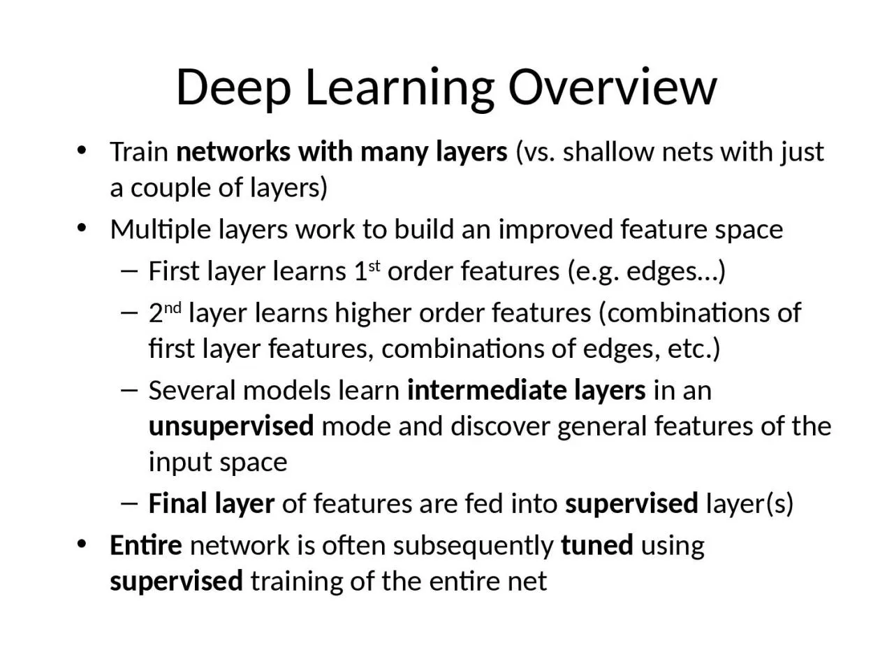
Deep Learning Overview Train - PowerPoint Presentation

1. Deep Learning OverviewTrain networks with many layers (vs. shallow nets with just a couple of layers)Multiple layers work to build an improved feature spaceFirst layer learns 1st order features (e.g. edges…)2nd layer learns higher order features (combinations of first layer features, combinations of edges, etc.)Several models learn intermediate layers in an unsupervised mode and discover general features of the input spaceFinal layer of features are fed into supervised layer(s)Entire network is often subsequently tuned using supervised training of the entire net

2. Deep Net Feature TransformationML ModelNew Feature SpaceOriginal FeaturesSupervisedLearningSupervised orUnsupervisedLearning

3. Face Recognition Example

4. Why Deep LearningBiological Plausibility – e.g. Visual CortexHighly varying functions can be efficiently represented with deep architecturesLess weights/parameters to update than a less efficient shallow representation (weight sharing)Sub-features created in deep architecture can potentially be shared between multiple tasks:Transfer or Multi-task learning

5. Deep Training DifficultiesVanishing Gradient – error attenuates as it propagates to earlier layers (f '(net)*(t-y))Leads to very slow training (especially at early layers)Need a way for early layers to do effective workInstability of gradient in deep networks: Vanishing or exploding gradientProduct of many terms, which unless “balanced” just right, is unstableEither early or late layers stuck while “opposite” layers are learningLong training times Many Local Minima of error functionAdvanced computing infrastructure is needed

6. Unsupervised Pre-TrainingThe first Deep-Learning approach (Deep Belief Networks 2006)Unsupervised Pre-Training uses unsupervised learning in the deep layers to transform the inputs into features that are easier to learn by a final supervised modelOften not a lot of labeled data available while there may be lots of unlabeled data. Unsupervised Pre-Training can take advantage of unlabeled data. Can be a huge issue for some tasks.

7. Greedy Layer-Wise TrainingTrain first layer using your data without the labels (unsupervised)Then freeze the first layer parameters and start training the second layer using the output of the first layer as the unsupervised input to the second layerRepeat this for as many layers as desiredThis builds the set of robust featuresUse the outputs of the final layer as inputs to a supervised layer/model and train the last supervised layer(s) (leave early weights frozen)Unfreeze all weights and fine tune the full network by training with a supervised approach, given the pre-training weight settings (optional)

8. Deep Net with Greedy Layer Wise TrainingML ModelNew Feature SpaceOriginal InputsSupervisedLearningUnsupervisedLearning

9. Greedy Layer-Wise TrainingGreedy layer-wise training avoids many of the problems of trying to train a deep net in a supervised fashionEach layer gets full learning focus in its turn since it is the only current "top" layer (no unstable gradient issues, etc.)Can take advantage of unlabeled dataWhen you finally tune the entire network with supervised training the network weights have already been adjusted so that you are in a good error basin and just need fine tuning. This helps with problems ofIneffective early layer learningDeep network local minimaTwo landmark approachesDeep Belief Networks (2006)Stacked Auto-Encoders (2007)

10. Auto-Encoders A type of unsupervised learning which discovers generic features of the data (self-supervised learning)Learn identity function by learning important sub-featuresCompression, etc. – Undercomplete |h| < |x|For |h| ≥ |x| (Overcomplete case more common in deep nets) use regularized autoencoding

11. Sparse Auto-EncodersUse more hidden nodes in the encoderUse regularization techniques which encourage sparseness (e.g. a significant portion of nodes have zero output for any given input)Penalty in the learning function for non-zero nodesWeight decayDe-noising Auto-EncoderStochastically corrupt training instance each time, but still train auto-encoder to decode the uncorrupted instanceImproved empirical results

12. Stacked Auto-EncodersBengio (2007) – After Deep Belief Networks (2006)Stack many (sparse) auto-encoders in succession and train them using greedy layer-wise trainingDrop the decode output layer each time

13. Stacked Auto-EncodersDo supervised training (can now only used labeled examples) on the last layer using final featuresThen do supervised training on the entire network to fine- tune all weights (optional)

14. Deep Belief Networks (DBN)Beginning of Deep Learning hype (2006) – outperformed kernel methods (SVMs) on MNIST – Also generativeUses Greedy layer-wise training but each layer is an RBM (Restricted Boltzmann Machine)RBM is a constrained Boltzmann machine withNo lateral connections between hidden (h) and visible (x) nodesSymmetric weights, different biasesTypically uses probabilistic logistic node, but other activations possible

15. RBM Sampling and Training Initial state typically set to a training example x (can be real valued)Sample in an iterative back and forth processP(hi = 1|x) = sigmoid(Wix + ci) = 1/(1+e-net(hi)) // ci is hidden node biasP(xi = 1|h) = sigmoid(W'ih + bi) = 1/(1+e-net(xi)) // bi is visible node biasContrastive Divergence (CD-k): the difference from the original training example to the relaxed version after k relaxation stepsThen update weights to decrease the divergenceTypically just do CD-1 (Good empirical results)

16.

17. Deep Belief Network TrainingGreedy layer-wise approachFirst train lowest RBM (h0 – h1) using RBM update algorithm (note h0 is x)Freeze weights and train subsequent RBM layersThen connect final outputs to a supervised model and train that modelFinally, unfreeze all weights, and fine tune as an MLP using the initial weights found by DBN trainingCan do execution as just the tuned MLP

18. Fully Supervised Deep LearningMuch recent success in doing fully supervised deep learning with extensions which diminish the effect of early learning difficulties (unstable gradient, etc.)Patience (now that we know it may be worth it), faster computers, use of GPUsMore efficient activation functions (e.g. ReLUs) in terms of both computation and avoiding f '(net) saturationPut some effort on weight initializationUse Dropout during trainingTraining using variations of Scaled Conjugate Gradient (SGD) that speed-up learning + Train in mini-batchesBatch normalization in hidden nodes: for every hidden node input (k):

19. Speed up variations of SGDAdaptive learning rate (LR) approaches:Standard MomentumNesterov Momentum – Calculate point you would go to if using normal momentum. Then, compute gradient at that point. Do normal update using that gradient and momentum.Rprop – Resilient BackProp, if gradient sign inverts, decrease it’s individual LR, else increase it – common goal is faster in the flats, there are variants that backtrack a step, etc.Adagrad – Scale LRs inversely proportional to the sum of past values – LRs with smaller derivatives are decreased lessRMSprop – Adagrad but uses exponentially weighted moving average, older updates basically forgottenAdam (Adaptive moments) – Momentum terms on both gradient and squared gradient

20. Convolutional Neural NetworksNetworks built specifically for problems with low dimensional grid-like local structure (e.g. images)Inspired from biological computations in visual cortex (visual pyramid)Neighboring pixels will have high correlations and local features (edges, corners, etc.), while distant pixels are un-correlatedNatural images have the property of being stationary, meaning that the statistics of one part of the image are the same as any other partCNNs enforce that a node receives only a small set of features which are spatially or temporally close to each other called receptive fields from one layer to the next (e.g. 3x3, 5x5), thus enforcing ability to handle local 2-D structure.Good for problems with local grid structure, but inappropriate for general learning with abstract features having no prescribed feature ordering or locality

21. Convolutional Neural NetworksTypical MLPs: fully connectivity between layersConvolutional nets (sparse connectivity + weight sharing):Nodes still do a scalar dot product (convolution) from the previous layer, but with only a small portion (receptive field) of the nodes in the previous layer – Sparse connectivityEvery node has the exact same weight values from the preceding layer – Shared parameters, tied weights, a LOT less unique weight values (regularization)Each node has it’s shared weight convolution computed on a receptive field slightly shifted, from that of it’s neighbor, in the previous layer – Translation invariance.Each node’s convolution scalar is then passed through a non-linear activation function (ReLU, tanh, etc.)Convolution is a simple weighted sum

22. Convolution Example

23. Convolution layersThe 2-d layers (grids) of nodes (or their outputs) in a CNN are called feature maps Each node in a feature map has the same weights, and each node connects to a different overlapping receptive field of the previous layer (stride parameter determines overlapping)Each feature map ‘scans’ previous layer to see where its feature occursLater layers could concern themselves with higher order combinations of features

24. Convolutional Neural NetworksC layers are convolutions, S layers pool/sampleOften starts with fairly raw features at initial input and lets CNN discover improved feature layer for final supervised learner – eg. MLP/BP

25. CNN StructureEach node in convolution layer is calculated for each receptive field in the previous layerDuring training the corresponding weights are always tied to be the sameThus a relatively small number of unique weight parameters to learn, although they are replicated many times in the feature mapEach node output in CNN is f(Σxw + b) (ReLU, tanh etc.)Multiple feature maps in each layerEach feature map should learn a different feature

26. Convolution layersThe 2-d layers (grids) of nodes (or their outputs) in a CNN are called feature maps Each node in a feature map has the same weights, and each node connects to a different overlapping receptive field of the previous layer (stride parameter determines overlapping)Each feature map ‘scans’ previous layer to see where its feature occursLater layers could concern themselves with higher order combinations of features

27. Sub-Sampling (Pooling)Sub-sampling (Pooling) allows number of features to be diminished, and to pool informationPooling replaces the network output at a certain point with a summary statistic of nearby outputsMax-Pooling common, also average pooling, stochastic pooling etc.Pooling smooths the data and reduces spatial resolution2x2 pooling would do 4:1 compression, 3x3 9:1, etcConvolution layer (C) followed by sub-sampling layer (S) and so onA fully connected MLP is added on the top of the final S layer.

28. Pooling Example (Summing or averaging)

29. CNN Examples

30. CNN weight sparsityConvolution layerEach feature map has one weight for each input and one biasA feature map with a 5x5 receptive field (filter) would have a total of 26 weights, which are the same coming into each node of the feature mapIf a convolution layer had 10 feature maps, then only a total of 260 unique weights to be trained in that layerSub-Sampling (Pooling) LayerAll elements of receptive field max’d, averaged, summed, etc. Result multiplied by one trainable weight and a bias added, then passed through non-linear function (e.g. ReLU) for each pooling nodeIf a layer had 10 pooling feature maps, then 20 unique weights to be trained

31. CNN TrainingCNNs trained with gradient-based methods (e.g. SGD) and cross-entropy loss function but with weight sharing in each feature mapGradients computed using back-propagationAdd (or average) the weight updates over the shared weights in feature map layersMini-batch trainingRandomized initial weights through entire network

32. CNN HyperparametersThe structure of the CNN is currently usually hand crafted with trial and error (cross-validation or simple validation error)Parameters to be determined:Number of layersSize of filters (receptive field)Receptive field overlapping (stride)Number of feature maps in convolution layers Connectivity between layers Activation functionsSize of pooling layersType of poolingFinal supervised layers etc

33. Example – LeNet-5 – MNIST Classification (the first CNN)

34. ILSVRC Image net Large Scale Vision Recognition Competition

35. Example CNNs Structures ILSVRC winnersNote Pooling considered part of the layer96 convolution kernels, then 256, then 384Stride of 4 for first convolution kernel, 1 for the restPooling layers with 3x3 receptive fields and stride of 2 throughoutFinishes with fully connected (fc) MLP with 2 hidden layers and 1000 output nodes for classes

36. Example CNNs Structures ILSVRC winners

37. CNN SummarySpecial purpose deep neural netInappropriate for general datasetsHigh accuracy for image applications – Breaking all records and doing it using just using just raw pixel features (no image preprocessing)!CNNs are effective when inputs are structured (grid-like)Tedius of hand-crafting and hyperparameter tuningLong training times (large computing infrastructure necessary)Pretrained networks (e.g VGG, ResNet) can be used as backbone and easily fine tuned to solve specific tasks (transfer learning).

38. TransformersVery successful on sequential data (e.g. Natural Language Processing Applications)Feedforward neural networksFound to be superior to Recurrent Neural Networks (LSTMs, GRUs) that have been used for training using sequential data.Transform a sequence to another sequence (e.g. language translation)Based on the idea of self-attentionInclude an encoder part and a decoder part

39. TransformersThe encoder part takes as input a sequence of vectors (e.g word embeddings) Encodes its position (positional encoding) produces an efficient internal representation of the sequence using: self-attention modules + MLPsThis representation is passed to the decoder that generates the ‘translated’ sequence. The self-attention module is based on the Query-Key-Value idea.

40. TransformersIn several applications the encoder part (self-attention + MLP) can also be trained solely (without the decoder) in a self-supervised manner.The encoder self-pretrained on huge datasets can be used as a backbone (eg. BERT, GPT) for several applications: just add and train a classification layer on top of the backbone to solve a specific problem (transfer learning)

41. Synthetic Data GenerationGiven a set of data object (eg. face images), generate synthetic samples that are ‘similar’ to the original ones (e.g. synthetic faces)Most popular approachesGenerative Adversarial Networks (GANs)Generator : takes input noise (sampled from the normal distribution) and generates synthetic dataDiscriminator: classifier that learns to discriminate between real and synthetic dataObjective: generator tries to ‘fool’ the discriminatorVariational Autoencoders (VAEs): autoencoders trained so that the ‘code vectors’ follow the Normal Distribution.