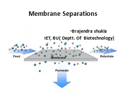
Brajendra shukla IET BU Deptt Of Biotechnology Membrane separations used in DSP Membrane separations Introduction Membranes are semipermeable barrier used for ID: 919742
Download Presentation The PPT/PDF document "Membrane Separations ..." is the property of its rightful owner. Permission is granted to download and print the materials on this web site for personal, non-commercial use only, and to display it on your personal computer provided you do not modify the materials and that you retain all copyright notices contained in the materials. By downloading content from our website, you accept the terms of this agreement.
Slide1
Membrane Separations -Brajendra shukla IET, BU( Deptt. Of Biotechnology)
Slide2Membrane separations used in DSP
Slide3Membrane separations: IntroductionMembranes are semi-permeable barrier used forParticle-liquid separationParticle-solute separationSolute-solvent separationSolute-solute separationApplications
Product concentrationProduct sterilizationSolute fractionation
Solute removal from solutions (desalination, demineralization)
Purification
Clarification
Slide4Factors utilized in membrane separationsSolute sizeElectrostatic chargeOther non-covalent interactionsDiffusivitySolute shape
Slide5Transport of material through a membraneDiffusion driven separationPressure driven separation
(convective transport)
Membrane module
Retentate
Permeate
Membrane
Membrane module
Retentate
Permeate
Membrane
Sweep
Feed
Feed
Slide6Dead-ended or conventional filtrationCross-flow filtration
Slide7Membrane materialsOrganic polymersPolysulfone (PS)Polyethersulfone (PES)Cellulose acetate (CA)Regenerated cellulosePolyamides (PA)
Polyvinylidedefluoride (PVDF)
Polyacrylonitrile
(PAN)
Inorganic materials
Glass
Metals
Ceramics
Layers of chemicals
Pyrolyzed
carbon
Slide8Membrane preparation by castingPrecipitation from vapour phaseThis is achieved by penetration of the precipitant through a polymeric film from the vapour phase, which is saturated with the solvent used.Precipitation by evaporationThe polymer is dissolved in a mixture of more volatile and less volatile solvents. As the more volatile component evaporates, the polymer precipitates to form the membrane.Immersion precipitation
This involves immersion of the cast film in a bath of non-solvent for coagulation of the membrane material.
Thermal precipitation
The polymer is precipitated from solution by a cooling step.
Slide9Other membrane making proceduresStretching: Involves stretching a polymer film at normal or elevated temperature in order to produce pores of desired size.Sintering: Powdered material is sintered by compression with/without heating to give microporous membranes.
Slip casting: Most inorganic membranes are prepared using this method.
The method involves coating repeated layers of uniform particles with decreasing sizes on porous support.
Slide10Other membrane making proceduresLeaching: Some inorganic membranes are prepared by leaching technique. Isotropic glass membranes are prepared by a combination of phase separation and acid leaching.Track etching: A homogeneous polymer film is exposed to laser beams or beams of collimated charged particles. This breaks specific chemical bonds in the polymer matrix.
The film is then placed in an etching bath to remove the damaged sections thus giving rise to
monodisperse
pores
Slide11Membranes: Structural classificationIsotropic
Anisotropic
Slide12Porous membranes
Isoporous
membrane
Microporous
symmetric
Microporous
asymmetric
Slide13Basic forms of membranesFlat sheet membraneTubular membraneHollow fibre membrane
Slide14Factors influencing the performance of a membraneMechanical strengthTensile strength, bursting pressureChemical resistancepH range, solvent compatibilityPermeability to different speciesPure water permeability, sieving coefficientAverage porosity and Pore size distribution
Sieving propertiesNominal molecular weight cut-off
Electrical properties
Membrane zeta potential
Slide15Driving force in membrane separationTransmembrane (hydrostatic) pressure (TMP)Concentration or electrochemical gradientOsmotic pressureElectrical fieldPartial pressurepH gradient
Slide16Membrane processes that separate primarily based on size (pressure driven)1 to 50 psi
10 to 100 psi
200 to 600 psi
Slide17Membrane processes that separate based on principles other than sizePervaporationSeparates a volatile or low-boiling-point liquid from a non-volatile liquid The driving force is a vacuum on the gaseous side of the membrane Tool for separation of liquid mixtures, especially dehydration of liquid hydrocarbons
Slide18Applications of pervaporationDehydration of ethanol–water azeotropeRemoval of water from organic solventsRemoval of organics from water
Slide19Membrane processes that separate based on principles other than sizeElectrodialysis (ED) Electrochemical process used to separate charged particles from an aqueous solution or from other neutral solutesA stack of membranes is used, half of them passing positively charged particles and rejecting negatively charged ones; the other half doing the opposite.
An electrical potential is imposed across the membranes and a solution with charged particles is pumped through the system.
Positively charged particles migrate toward the negative electrode, but are stopped by a positive-particle-rejecting membrane
Negatively charged particles migrate in the opposite direction with similar results
Slide20Electrodialysis (ED)
Slide21FluxThroughput of material through a membraneFlux depends onApplied driving forceResistance offered by membrane Fouling Increase in membrane resistance during a processThe decline in flux through a membrane with time in a constant force membrane process is due to fouling
Flux
Time
Decline in flux due to fouling in a
constant driving force membrane
separation
Pressure
Time
Fouling in constant flux
membrane separation
Slide22Fouling of membranes
Slide23Membrane element and moduleMembrane element refers to the basic form of the membrane:
Flat sheet
Hollow
fibre
Tubular
Membrane module refers to the device which houses the membrane element:
Stirred cell module
Flat
sheet tangential flow (TF) module
Tubular
membrane module
Spiral wound membrane module
Hollow
fibre membrane module
Slide24Membrane modules
Stirred cell unit
Arrangement flat sheet TF module
Small scale flat sheet TF module
Pilot plant scale flat sheet TF module
Slide25Stirred cell
Research and small-scale manufacturing
Used for microfiltration and
ultrafiltration
Excellently suited for process development work
Slide26Flat sheet tangential flow module
Similar plate and frame filter press
Alternate layers of membranes, support screens and distribution chambers
Used for microfiltration and
ultrafiltration
Slide27Spiral flow membrane moduleFlat sheet membranes are fused to form an envelop
Membrane envelop is spirally wound along with a feed spacer
Filtrate is collected within the envelope and piped out
Slide28Spiral wound module
Slide29Slide30Millipore spiral wound module
Slide31Tubular membrane module
Cylindrical geometry; wall acts as the membrane
Tubes are generally greater than 3 mm in diameter
Shell and tube type arrangement is preferred
Flow behaviour is easy to
characterise
Tubular membranes are used for all types of pressure driven separationsTubular modules are widely used where it is advantageous to have a turbulent flow regimeAdvantages
Low fouling and hence relatively easy cleaning
Easy handling of suspended solids & viscous fluids
Ability to replace or plug a damaged membrane.
Disadvantages
High capital cost
Low packing density
High pumping costs
High dead volume
Tubular membrane module
Slide33Section of tubular module
Large scale tubular module
Slide34Hollow fibre membrane module
Similar to tubular membrane module
Tubes or fibres are 0.25 - 2.5 mm in diameter
Fibres are prepared by spinning and are potted within the module
Straight through or U configuration possible
Typically several fibres per
module
Slide35Hollow fibre membrane
Slide36Plate and frameSpiral woundTubular
Hollow fiber
Packing density
30 – 500
200 – 800
30 – 200
500 – 9000
Resistance to fouling
Good
Moderate
Very good
Poor
Ease of cleaning
Good
Fair
Excellent
Poor
Relative costHigh
LowHighLow
Main ApplicationsD, RO, PV, UF, MFD, RO, GP, UF, MF
RO, UFD, RO, GP, UF
Comparison of different membrane modules
Slide37TypeFluid flow regime
Membrane area/module volume
Mass transfer coefficient
Hold-up volume
Special remarks
TF flat sheet
Laminar- turbulent
Low
Low to moderate
Moderate
Can be dismantled and cleaned
easily
Spiral wound
Laminar
Moderate
Low
Low
High pressures cannot be
used
Hollow fibre
Laminar-turbulent
High
Low to moderate
Low
Susceptible to fibre
blocking
Tubular
Turbulent
Low
Moderate to high
Moderate to high
Flow easy to
characterize
Excellently suited for basic membrane studies.
Operating characteristics of membrane modules
Slide38Flow patterns in membrane modules
Slide39Membrane characterizationThe performance of a membrane process depends on the properties of the membrane:Mechanical strength
Tensile strength, bursting pressure
Chemical
resistance
pH
range, compatibility with solvents
Permeability to different
species
Pure
water permeability, gas permeability
Average porosity and pore size distribution
Sieving
properties
Nominal
molecular weight cut-off
Electrical properties
Membrane zeta potential
Slide40UltrafiltrationGeneral Industrial Uses:Concentration of macromoleculesPurification of solvent by removal of solutesFractionation of macromoleculesClarification
Retention of catalystsAnalysis of complex solutions for specific solutes
Bioprocess Applications
:
Fractionation of biological macromolecules e.g. proteins, DNA
Concentration of polymer solutions
Removal of LMW solutes from protein solutions
Removal of cells and cell debris from fermentation broth
Virus removal from therapeutic products
Harvesting of biomass e.g., cells and sub-cellular products
Membrane bioreactors
Effluent
treatment
Slide41Ultrafiltration membranesPores: 10 to 1000 AngstromsGenerally anisotropic (skin layer 0.2 to 10 micron thick)Properties of an ideal ultrafiltration
membrane:
High hydraulic permeability to solvent
Sharp “retention cut-off” properties: The membrane must be capable of retaining completely nearly all the solutes above some specified value, known as the molecular cut-off (MWCO
)
Good mechanical durability
Good chemical and thermal stability
Excellent manufacturing reproducibility and ease of manufacture
Slide42Sharp and diffuse cut-off membranes
Slide43Ultrafiltration: Pore flow model
J
v
=
Permeate flux
m
=Membrane
porosity
d
p
=
Average pore diameter
P =
Transmembrane pressure
=Viscosity
Lp =Average pore length
Hagen-
Poiseuille’s law for permeate flux
of pure solvent
P
i
and
P
o
inlet and outlet pressures on the feed side
P
f
is the pressure on the filtrate side
The pressure drop for a
Cross flow membrane module
Slide44Ultrafiltration: Flux equationsPore flow model: UF of solvent
Resistance model: UF of solvent
Osmotic pressure model: UF of solution
R
m
= membrane hydraulic
resistance
R
cp
= resistance due to concentration polarization
R
g
= gel layer resistance
R
m
= membrane hydraulic resistance
Slide45Concentration polarization
Slide46Concentration polarization model UF of solution
Material balance in a control volume within the concentration polarization layer at steady state
Upon integration with boundary conditions
C=
C
w
at x=0 and C=
C
b
at x=
δ
b
we get concentration polarization equation for partially rejected solutes
For total solute rejection
i.e
, C
p
= 0
When
C
w is equal to the gelation concentration, there will be no further increase in the value of
Cw
Hence we write gel polarization equation as
Slide47Effect of transmembrane pressure on permeate fluxAt constant TMP the permeate flux decreases as the feed concentration increases
When
C
w
= C
g
the permeate flux is independent of the TMP
Slide48ProblemA protein solution (conc, 4.4 g/l) is being ultrafiltered using a spiral wound membrane module which totally retains the protein. At a certain transmembrane pressure the permeate flux is 1.3x10
-5 m/s. The diffusivity of the protein is 9.5 x 10
-11
m
2
/s while
the wall concentration at this operating pressure is estimated to be
10 g/l.
Predict the thickness of the boundary layer.
If the permeate flux is increased to 2.6 x 10
-5
m/s while maintaining the same hydrodynamic conditions within the membrane module, what is the new wall concentration?
Slide49Where there is total retention we can use the equationThis equation can be written as The mass transfer coefficient is given by ThereforeWhen
Jv
is increased to 2.6 x 10
-5
m/s and
k
remains the same, the wall concentration can be obtained from the concentration polarization equation for totally retained solute
Slide50Effect of feed concentration on permeate flux
TMP
J
v
C
b
J
lim
ln
C
b
C
s
or
C
g
k
For a given feed concentration, the limiting flux increases with increases in mass transfer coefficient
Permeate flux decreases as the feed concentration is increased
Slide51Mass transfer coefficient (k) Affects back-diffusion of accumulated solute
Measure of the hydrodynamic conditions within the module
k
= (
D/
b
)
Mass
transfer coefficient can be measured experimentally
Plot of limiting flux versus log of feed concentration
Plot of sieving parameter versus (
J
v
/
k) Mass
transfer coefficient can be estimated using heat-mass transfer analogyDimensionless equations: Sherwood number as function of Reynolds number and Schmidt number
Slide52Schmidt number = Momentum transfer/Mass transfer
Reynolds number = Inertial forces/Viscous forces
Sherwood number = Total mass transfer/Diffusive mass transfer
Mass transfer correlations
Peclet
number = Convective mass transfer / Diffusive mass transfer
Grashof
number = Gravitational forces/ Viscous forces
Froude number =
Interial
forces/ Gravitational forces
Slide53Mass transfer correlationsFully developed laminar flow (i.e. Re < 1000) in tubular membrane
Turbulent flow (i.e.
Re
> 2000) in tubular membrane
Graetz
-Leveque
Dittus-Boelter
Fully developed laminar flow
Porter
Shear rate at the wall
= 8
u
l
/
d
for
tubes
= 6
ul /
b for rectangular channels (b = channel depth)
Slide54Problem: Shear-Induced DiffusivityShear-induced diffusivity is 3 x 10⁻⁷ cm2/s.
Hydrodynamic diffusivity is 2
x10
-9
cm
2
/s.
Shear-induced diffusivity
is about 150 times larger.
Compare hydrodynamic and shear-induced diffusivity values for
a 1-mm
particle at a shear rate of 1,000
s
-1
. Assume the value of
α to be 0.03 for ultra filtration processes
Slide55Problem:
Calculate the mass transfer coefficient for ultrafiltration of milk at 50
o
C employing tubular membrane system with the following configurations:
Pore diameter of 1.25 cm; Length = 240 cm;
Number of channels = 18;
superficial velocity = 200 cm/sec;
Pressure drop over length = 2 kg/cm
2
.
The physical properties of milk are as follows:
Density = 1.03 g/ml;
viscosity 0.008 g/cm/sec;
Diffusivity = 7.0 x 10
-7
cm
2
/sec.
The bulk protein concentration is 3.1% and the gel protein concentration is 22%. Assume turbulent regime for the process and make use of
Dittus-Boelter
correlation
Slide56= 32188
= 11096
For calculating Sherwood number in turbulent
flow
regime (i.e
.
Re
> 2000) in tubular
membrane,
Dittus-Boelter
correlation can be used
= 2008
Slide57Now for calculating mass transfer coefficient k we will make use of the Sherwood number
To calculate the flux for the process
Slide58Calculate the mass transfer coefficient for
ultrafiltration
of milk at 50
o
C employing tubular membrane system with the following configurations:
Pore diameter of 1.25 mm; Length = 240 cm;
Number of channels = 18;
superficial velocity = 200 cm/sec;
Pressure drop over length of tube = 2 kg/cm
2
Shear
rate at wall = 7272.0 /sec
The physical properties of milk are as follows:
Density = 1.03 g/ml;
viscosity 0.008 g/cm/sec;
Diffusivity = 7.0 x 10
-7
cm
2
/sec.
The bulk protein concentration is 3.1% and the gel protein concentration is 22%. Assume turbulent regime for the process and make use of
Dittus-Boelter
correlation
Slide59Effect of hydrodynamic parameters on permeate flux
Slide60Enhancement of permeate fluxBy increasing the cross-flow rate By creating pulsatile flowBy pressure pulsingBy creating oscillatory flowBy flow obstruction using bafflesBy generating Dean vorticesBy generating Taylor vortexBy gas-sparging
into the feed
Slide61Dean vorticesDean vortices are helicoidal flows created by centrifugal forces in curved channelsCoiled or helically twisted tubular membranes Enhance solute back transfer away from the membrane Effective for enhancing permeate flux by depolarization of the solute layer on the membrane
Slide62Dean vorticesDean vortices are secondary tangential flows that create a self-cleaning flow mechanism when induced within a cross-flow filtering systemThe general principle of this technologyto design, develop and use these tangential flows to sweep around a curve to “clean” the membrane, leading to enhanced filter performance and longer membrane life
Slide63Taylor VortexSpecialised type of Couette flowWhen the angular velocity of the inner cylinder is increased above a certain thresholdCouette flow becomes unstable and a secondary steady state characterized by axisymmetric toroidal vortices
Plasma collection from donors in transfusion centers by microfiltration
Slide64Plasma cell filter for plasma collection from donors with a rotating cylindrical membraneDYNAMIC FILTRATION
Biodruckfilter
(
sulzer
AG, Winterthur, Switzerland)
http://www.sulzer.com
.
Rotary
biofiltration
device (
Membrex
Inc.) and merged into GE
Osmonic
(
www.gewater.com)
Slide65Rotating Disk ModulesMSD system (Westfalia
Separator, Aalen, Germany)
Multishaft
systems with overlapping rotating membranes
The MSD system features 31-cm-diameter ceramic membranes on eight parallel shafts located on a cylinder for a membrane area of 80 m
2
All disks rotate at the same speed and are enclosed in a cylindrical housing
The membrane shear rate is unsteady and reaches a maximum in the overlapping regions
Slide66Rotating disk dynamic filtration system (Pall Corp., Massachusetts, USA) www.pall.comDyno (Bokela GmbH, Karlsruhe, Germany) www.bokela.comOptifilter CR (Metso
Paper, Raisio, Finland)
www.metso.com/
Multi-disk system (
SpinTek
, Huntington, CA, USA)
www.spintek.com
MSD system (
Westfalia
Separator, Aalen, Germany)
www.westfalia-separator.com
Rotostream
(
Canzler
, Dueren, Germany)
http://www.sms-vt.com/index.phpMultishaft disk (MSD) system (Hitachi Ltd.) www.hitachi.com
Self Cleaning Filtration, (novoflow, Oberndorf
, Germany) http://www.novoflow.com/en/home
Rotating Disk Modules
Slide67Flux Enhancement by Pulsatile FlowsAnother method for enhancing permeate flux and mass transfer without using very high fluid velocity Consists of superposing flow and pressure pulsations at the membrane inlet with a piston-in-cylinder system or special pumps such as modified roller pumps
Pulsatile blood flow to enhance gas transfer in membrane blood oxygenators
Slide68RetrofiltrationTechnique for reducing membrane fouling by pressurizing the permeate above retentate pressure in order to inject permeate into retentate and clean the poresBackwashingBackpulsing
Slide69Vibratory shear-enhanced processingSchematic of the vibratory shear-enhanced processor (VSEP) pilot series L with a single membrane oscillating around its vertical axis
Vibratory shear-enhance processing (VSEP) (
New Logic Research, Inc.
)
www.vsep.com
PallSep
Vibrating Membrane Filter (Pall Corporation)
http://www.pall.com
Slide70Solute transmission through UF membranesAmount of solute going through an UF membrane can be quantified in terms of the membrane intrinsic rejection coefficient (Ri) or intrinsic sieving coefficient (Si
):
C
w
is difficult to determine and hence it is more practical to use the apparent rejection coefficient (
R
a
) or the apparent sieving coefficient (
S
a
):
Slide71Factors influencing the retention of a solute by membrane Primary variableSolute diameter to pore diameter ratioAlso depends onSolute shapeSolute chargeSolute compressibilitySolute-membrane interactions
Operating conditions
The amount of solute going through the membrane can be quantified in terms of
intrinsic rejection coefficient (
R
i
) and intrinsic sieving coefficient (S
i
)
Slide72Rejection coefficient:Older theory new theory
for
< 1
for
1
= (
d
i
/
d
p
)=solute-pore diameter ratio
In other words, R
a is constant for a solute-membrane system.
It is now recognised that rejection coefficients depend on operating and environmental parameters such as
pHIonic strengthSystem hydrodynamicsPermeate flux
Slide73Sieving coefficients
Intrinsic sieving coefficient
Depends on solute-membrane system
Depends on physicochemical parameters such as pH and ionic strength
Depends on permeate flux
Apparent sieving coefficient
Depends on solute-membrane system
Depends on physicochemical parameters such as pH and ionic strength
Depends on permeate flux
Depends on system hydrodynamics
Slide74Effect of permeate flux on intrinsic sieving coefficient
S͚
Slide75Effect of permeate flux and mass transfer coefficient on apparent sieving coefficient
Slide76Determination of intrinsic sieving coefficient and mass transfer coefficient
Slide77ProblemThe intrinsic and apparent rejection coefficients for a solute in an ultrafiltration process were found to be 0.95 and 0.63 respectively at a permeate flux value of 6 x 10⁻³ cm/s.What is the solute mass transfer coefficient?
Slide78Solution:
Sa
= 1-R
a
= 1-0.63 = 0.37
S
i
= 1-R
i
= 1-0.95 = 0.05
Slide79Solute fractionationFor fractionation of a binary mixture of solutes, it is desirable to achieve maximum transmission of the solute desirable in the permeate and minimum transmission of the solute desirable in the retentate.
Enhancement of
fractionation
pH
optimization
Feed
concentration optimization
Salt
concentration optimization
Membrane
surface pre-treatment
Optimization
of permeate flux and system hydrodynamics
Selectivity parameter
Slide80ProblemA feed solution (10 g/l) of dextran (MW=505 kDa) is ultrafiltered through a 25 kDa MWCO Membrane. The pure water flux values and the dextran UF permeate flux
values at different TMP are given below
The osmotic pressure is given by the following correlation
where
Δπ
is in dynes/cm
2
and
C
w
is in %w/v.
Calculate the membrane resistance and the mass transfer coefficient for
dextran
assuming that
Rg and Rcp are negligible
Δ
P (kPa)
Pure water flux (m/s)Jv (m/s)
309.71x10⁻⁶
6.24x10-6401.23 x 10
-57.08x10⁻⁶
501.57x10⁻⁵
7.63x10-6601.87x10
-58.02x10⁻⁶
Slide81SolutionThe MWCO of the membrane is 25 kDa while the MW of dextran is 505 kDa. Hence we can safely assume that
dextran is totally retained. Pure water
ultrafiltration
is governed by
R
m
= 3.33 x 10
9
Pa.s
/m
Slide82We also know that
Since
R
cp
and
R
g
are negligible the equation becomes
Using the above equation we can calculate the osmotic pressure for every value of
transmembrane
pressure
Δ
P
(
kPa
)
Pure water flux (m/s)J
v (m/s)Δ
π (kPa)Δπ (dynes/cm
2)Cw(%w/v)
Cw(g/l)K
(m/s)309.71x10
-66.24x10-6
9.22922087.63
76.313.07x10-6
401.23 x 10⁻⁵
7.08x10-616.42
16423610.04
100.43
3.7x10-650
1.57x10-57.63x10-6
24.5924592111.99
119.94
3.07x10-660
1.87x10-58.02x10
-633.29332934
13.61136.08
3.07x10
-6
Slide83The correlation for osmotic pressure given in the problem can be rearranged to Using the above equation the wall concentration at different TMP can be calculated
The mass transfer coefficient in an UF process with total solute retention is given by
Rearranging the equation we get
Slide84MicrofiltrationMicrofiltration separates micron-sized particles from fluids The modules used for microfiltration are similar to those used in ultrafiltration Microfiltration membranes are microporous and retain particles by a purely sieving mechanism
Microfiltration can be operated either in dead-ended (normal flow) mode or cross-flow mode
Typical permeate flux values are higher than
ultrafiltration
processes even though the processes are operated at much lower TMP
Slide85Applications of microfiltrationCell harvesting from bioreactorsVirus removal for solutionsClarification of fruit juice and beveragesRemoval of cells from fermentation mediaWater purificationAir filtration
Sterilization
Slide86The permeate flux in microfiltration
J
v
= Permeate flux
P
= Pressure difference across the membrane
R
M
= Membrane resistance
R
C
= Cake resistance
= Liquid medium viscosity
The cake resistance
r
= Specific cake resistance
V
S
= Volume of cake
A
M
= Area of membrane
For micron sized particles,
r
is given by
= Porosity of cake
d
s
=
Mean particle diameter
Slide87Problem: Microfiltration of bacteriaBacterial cells having 0.8 micron average diameter are being microfiltered in the cross-flow mode using a membrane having an area of 100 cm2. The steady state cake layer formed on the membrane has a thickness of 10 microns and a porosity value of 0.35. If the viscosity of the filtrate obtained is 1.4 cP, predict the volumetric premeate flux at a
transmembrane pressure of 50 kPa
.
When pure water of viscosity 1
cP
was filtered through the same
transmembrane
pressure, the permeate flux obtained was 10
-4
m/s
Slide88For pure water filtration the flux is written as
The specific cake resistance of the bacterial cell cake can be calculated
from
The cake resistance
R
c
can be calculated from
Solution
Slide89The permeate flux can be calculated from = 6.58 x 10⁻⁵
m/s
Slide90DialysisThe mode of transport in dialysis is diffusionSeparation occurs because Small molecules diffuse more rapidly than larger onesAlso due to the degree to which the membrane restricts transport of molecules usually increases with solute size
Membrane
Bulk concentration
on downstream side (
C
2
)
Boundary layers
Concentration profile in dialysis
Bulk concentration on upstream side (
C
1
)
Slide91The rate of mass transport or solute flux (N) is directly proportional to the difference in concentration (C) at the membrane surfaces
S
is a dimensionless solute partition coefficient
D
eff
is the effective diffusivity of the solute within the membrane
d
is the membrane thickness
D
eff
and
d
can be combined and termed the membrane mass transfer coefficient (
K
M
) for a given membrane-solute system
Dialysis
Slide92K
O
= the overall mass transfer coefficient
K
1
and
K
2
are the mass transfer coefficients on the upstream and downstream sides
In terms of mass transfer coefficient
C
1
and
C
2
are the upstream (feed) and downstream (
dialysate
) concentrations
The membrane resistance alone seldom governs the overall mass transport. The liquid boundary layers on either side of the membrane also contribute to resistance to transport
R
O
= the overall resistance
R
1
= the resistance on the upstream surface
R2 = the resistance on the downstream surface
Slide93Hollow fiber dialyser
C
1
C
2
C
3
C
4
Co-current flow
Counter-current flow
C
1
C
3
C
2
C
4
Feed
Dialyzing solution (sweep stream)
Dialysate
Product
Feed
Dialyzing solution (sweep stream)
Dialysate
Product
Slide94Co-current and counter-current dialysis
Log-mean
concentration
difference (
∆
C
lm
)
Co-current
Counter-current
Length of membrane
Conc.
Feed side
Dialysate
Conc.
Length of membrane
Feed side
Dialysate
Slide95Co-current flow
Co-current operation is preferred when liquid flow causes significant pressure drop between inlet and outlet side
Generally in co-current mode membrane utilization is incomplete
Slide96Counter-current flow
Counter current mode ensures uniform
gradient and hence uniform solute flux
Counter current dialysis is most commonly
used as it ensures full membrane utilization
Slide97Co-current flow
Counter-current flow
C
1
C
3
C
3
C
4
C
1
Dialysis modes
C
4
Slide98Applications of dialysisRemoval of acid or alkali from productsRemoval of alcohol from beer (to make alcohol free beer)Removal of salts and low molecular weight compounds from solutions of macromoleculesConcentration of macromoleculesDialysis provides a tool for controlling the chemical species within a reactor
Purification of biotechnological products
Haemodialysis
Slide99The figure below shows a completely mixed dialyser unit. Plasma having a glutamine concentration of 2 kg/m3 is pumped into the dialyser at a rate of 5x10⁻⁶ m3/s and water at a flow rate of 9 x 10⁻⁶ m
3/s is used as the dialysing
fluid. If the membrane mass transfer coefficient is 2 x 10
-4
m/s and the membrane area is 0.05 m
2
,
calculate the steady state concentrations of glutamine in the product and
dialysate
streams.
Problem
Slide100SolutionThe overall material balance for glutamine gives ------- (a)
The glutamine concentration flux per unit area can be obtained using equation
The amount of glutamine in of the
dialysate
should be equal to the product of the concentration flux and area:
The amount of glutamine in the
dialysate
= Q
2
C
4
, therefore
------- (b)
Solving the two equations simultaneously, we get:
C2 = 1.027 kg/m3 C
4 = 0.541 kg/m3
Slide101Packed bed adsorption has several major limitationsHigh pressure dropIncrease in pressure drop during operationColumn blinding by proteinsDependence on intraparticle diffusion for the transport of proteins to their binding sites
High process times (due to iv)High flow rates cannot be used
High recovery liquid volume
Radial and axial dispersion resulting from the use of
polydisperse
media
Problems associated with scale-up
Slide102Advantages of membrane adsorbers Low process timeLow recovery liquid volumePossibility of using higher flow ratesLower pressure dropLess column blinding
Ease of scale-upFewer problems associated with validation (if a disposable membrane is used)
Slide103Comparison of solute transport in particulate packed bed and membrane adsorbers
Slide104Slide105Different types separation chemistries are used in membrane adsorptionAffinity bindingIon-exchange interactionReverse phase and hydrophobic interaction
Size exclusion based separation using membrane beds has not yet been feasible
Slide106Membrane adsorptionMembrane adsorption processes are carried out in two different modes Pulse Step Based on the membrane geometry, three types of membrane adsorbers are used:Flat sheetRadial flow
Hollow fibre
Slide107Operation of flat sheet membrane adsorber
Slide108Operation of hollow fibre membrane adsorber
Slide109δ
m
θ
C
θ
D
Diffusion and convection times in
membrane adsorption
Reynolds number of the fluid flowing through
the membrane pores
u
s
= superficial velocity (m/s)
d
pore
= average pore diameter (m)
v
= kinematic viscosity (m
2
/s)
ε
= porosity (-)
Time taken for solute to diffuse
from central line to the pore wall
Residence time of solute moving
along central line through a pore
d
pore
Slide110An adsorptive membrane has a thickness of 2 mm and a diameter of 5 cm. The porosity of the membrane is 0.75 and the tortuosity is 1.5. The pore diameter was estimated to be 2 x 10⁻⁶ m. If we are to use this membrane for adsorption of a DNA fragment (diffusivity = 9.5 x 10⁻¹² m2/s) from an aqueous solution, what is the maximum solution flow rate that can be used? Assume that the flow through the pores is laminar
Problem: Membrane adsorption of DNA
Slide111Area of the membrane = 1.964 x 10⁻³ m2The superficial velocity is given by The convection time can be obtained fromDiffusion time can be calculated using
For total capture of DNA θ
C
>
θ
D
. Therefore
The solution flow rate should be lower than 2.098 x 10
-5
m
3
/s.
Solution
Slide112ChromaSorb™ Membrane Adsorber (Millipore)
Single-use, flow-through anion exchanger designed for the removal of trace impurities including host cell protein (HCP), DNA,
endotoxins
and viruses from monoclonal antibody or other protein
feedstocks
.
Slide113Sartobind
™ Membrane
Adsorber
(Sartorius)
Slide114Schematic representation of membrane
adsorber
and the operations of one purification cycle
Slide115Liquid membrane technologyLiquid membrane extraction involves the transport of solutes across thin layers of liquid interposed between two otherwise miscible liquids There are two types of liquid membrane processes:Emulsion liquid membrane (ELM) processesSupported liquid membrane (SLM) processes
Slide116Liquid surfactant membrane process
Slide117Supported liquid membrane
Slide118Schematic diagram of the membrane emulsification process
Slide119Limitations1. Film diffusion2. Pore diffusion3. Binding kinetics
Limitations
1. Film diffusion
3. Binding kinetics
Slide120Reverse OsmosisIntroductionReverse OsmosisReverse Osmosis Equipment
Slide121IntroductionIn RO, the goal is usually to remove a solute from solution by passing the solvent through the membrane and leaving the solute in a concentrated retentate (reject) streamNote that this is a continuous process, unlike filtration; purified water is produced continuously
Slide122Advantageslow energy consumptionhigh removal of solute in one stageno components added (such as absorbing gas or extracting liquid)no phase changelow capital costseasy, modular, installation
Slide123DisadvantagesMembrane life (hopefully 3-5 years)Fouling Pretreatment costs (removal of suspended solids, fouling materials)Relatively low concentration of solutesIn order to understand and to predict membrane performance it is necessary to have transport equations that describe the transport of solvent and solute through the membraneIn all membrane processes, we are looking at relationships between forces (driving forces) and fluxes;
[Class: you name some examples of these relationships that you already know.]
Slide124Osmotic PressureThermodynamic property of a solution which represents how different a solution is compared to a pure solvent in terms of the pressure required to bring the solution up to the same chemical potential (ie., in equilibrium with) pure solvent what this means, practically, is that osmotic pressure acts against the pressure driving force for transport across a membrane.This osmotic pressure can be 'looked up' in a book - a thermodynamic property.A reasonable approximation of osmotic pressure is the
Van't Hoff Eqn
where n is the kmol of solute per
V
m
m
3
of pure solvent, which is the same as the molar concentration,
ci
Slide125Osmotic pressure
For concentrated solutions of uncharged solutes correlations
involving series of virial coefficients
are used
van’t
Hoff equation
The osmotic pressure difference across a
membrane is given by
Slide126Slide127Summary of the transport equationsSolvent flux
Pure water flux
Solute Flux
Concentration Polarization
Material Balance on Solute
Slide128THANK YOU
-
Brajendra