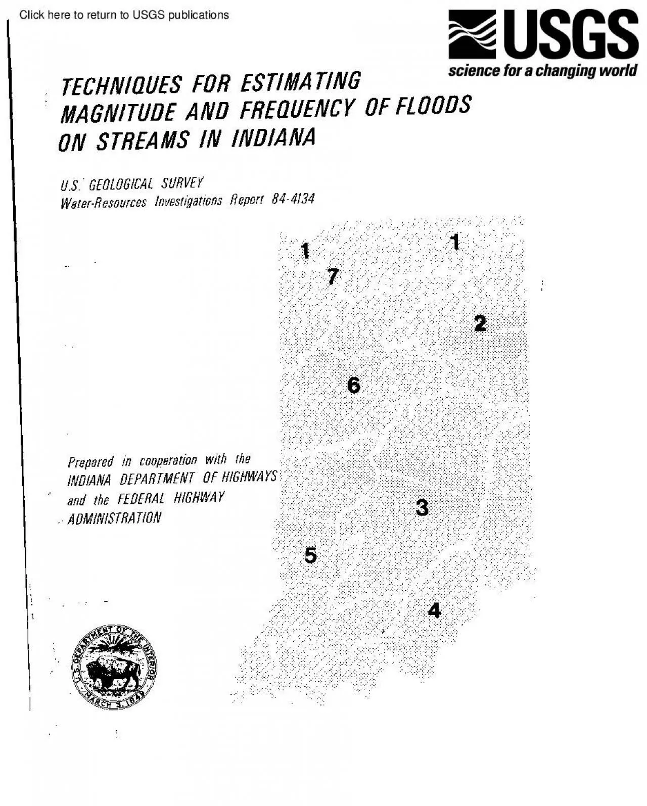
TECHNIQUES FOR ESTIMATING 146 h4AGNlTUDE AND FREQUENCY OF FLOODS ON S - PDF document

1 : TECHNIQUES FOR ESTIMATING ’ h4AGN
: TECHNIQUES FOR ESTIMATING ’ h4AGNlTUDE AND FREQUENCY OF FLOODS ON STREAIWS IN INDIANA U.S. GEOLOGICAL SURVEY Water-Resources Investigations Report 84-4134 Prepared in INDIANA DL ,,__. ._, ,_.,_ 0272-101 REPORT DOCUMENTATION 1. wPORT NO. 2. Recipient’s Accession No. PAGE 1.

2 Title and Subtitle 5. Report Date Te
Title and Subtitle 5. Report Date Techniques for Estimating Magnitude and Frequency of 1984 6. r. Author(s) 8. Performing Organization Rept. No. Dale R. Glatfelter USGS/WRI 84-4134 9. Performing Organization Name and Address 10. Pmiect/Task/Work Unit No. J.S. Geological Survey,

3 Water Resources Division 11. Contract(C
Water Resources Division 11. Contract(C) or Grant(G) No. 5023 Guion Suite 201 CC) Indianapolis, Indiana 46254 (‘3 12. Sponsoring J.S. Geological Survey, Water Resources Division Final 5023 Guion Suite 201 Indianapolis, Indiana 46254 14. Supplementary Notes Prepared in coope

4 ration with the Indiana Department of Hi
ration with the Indiana Department of Highways and the Federal Highway Administration 16. Abstract (Limit: 200 words) Nethods for estimating magnitude 25, 50, and years was developed for each area. The equations are valid for unregulated and nonurban streams. Significant basin characte

5 ristics in the equations are drainage ar
ristics in the equations are drainage area, channel length, channel slope, 45 percent. A rainfall-runoff model was used to extend the length of record at 11 sites on small streams. Flood-frequency data from the synthetic peaks and from the observed peaks were 17. Oocumeti. Analysis a.

6 Descriptors *Flood frequency, *Flood p
Descriptors *Flood frequency, *Flood peak, *Rainfall-runoff relationships, *Regional analysis, *Regression analysis, Flood recurrence interval, Frequency analysis, Indiana, Model studies, Regulated flow, Small watersheds, Statistical analysis, Stream discharge b. Identifiers/Open-Ended

7 Terms Basin characteristics, Magnitude
Terms Basin characteristics, Magnitude and frequency, Synthesis of discharge, Wabash River c. COSATI Field/Group b-l Y7tSon on alsvn. is repor?, may be purchased from: 19. Security Class (This Report) 21. No. of Pages Unclassified Open-File Services Sect., Western Distribution 110 Box

8 25425, Federal Ctr., Denver, 29. Secur
25425, Federal Ctr., Denver, 29. Security Class (This Page) 22. Price Unclassified Sea Instructions on Reverse (Formerly NTIS-35) Department of Commerce TECHNIQUES FOR ESTIMATING MAGNITUDE AND FREQUENCY OF FLOODS ON STRFAMS IN INDIANA By Dale R. Glatfelter U.S. GEOLOGICAL SURVEY Wate

9 r-Resources Investigations Report 84-413
r-Resources Investigations Report 84-4134 Prepared in cooperation with the INDIANA DEPARTMENT OF HIGHWAYS and FEDERAL HIGHWAY ADMINISTRATION Indianapolis, Indiana 1984 UNITED STATES DEPARTMENT OF THE INTERIOR WILLIAM P. CLARK, Secretary GEOLOGICAL SURVEY Dallas L. Peck, Director For addi

10 tional information write to: District Ch
tional information write to: District Chief U.S. Geological Survey 6023 Guion Suite 201 Indianapolis, Indiana 46254 Copies of this report can be purchased from: Open-File Services Section Western Distribution Branch U.S. Geological Survey Box 25425, Federal Center Denver, Colorado 80225

11 (Telephone: [303] 234-5888) 2 3 3 1
(Telephone: [303] 234-5888) 2 3 3 18 18 20 22 33 24 38 39 Figures I-i0. 1. 2. :: 5. I * 8. 9* 10. ILLUSTRATIONS Maps showing: Page Locations of streamflow data-collection sites............. 12 Areas for selecting flood-frequency estimating equations.. 14 NJean annual

12 precipitation, 1941-YO.................
precipitation, 1941-YO........................ 15 Two-year, 24-hour precipitation . ..*................. 16 Major hydrologic soil groups . I? Climatic factor a2 for estimating synthetic Q2 at Climatic factor aI0 for estimating synthetic Q10 at a rainfall-runoff station . 29 Clim

13 atic factor az5 for estimating syntheti
atic factor az5 for estimating synthetic Qz5 at a rainfall-runoff station . 30 Climatic factor aso 31 Climatic factor alOO for estimating synthetic Qloo at a rainfall-runoff station . ..a.............. 32 -iii- TABLES Table 1. 2. 3- 4. 5. 8 .,. 9* Page Equations for esti

14 mating magnitude and frequency of floods
mating magnitude and frequency of floods on 4 Statistics of logarithms of annual peaks...................... 42 Selected basin characteristics of gaging stations and partial-record sites ..*..................................... 60 T-year peak discharges at gaging stations and 104 Flo

15 od magnitude and frequency on the Wabash
od magnitude and frequency on the Wabash River, natural and regulated flow l . 108 Results from calibration of the rainfall-runoff model......... 26 Data 33 Equations used to combine observed and synthetic estimates of QT at rainfall-runoff stations 35 IO. Standard errors of estima

16 te of Qloo for area equations and equati
te of Qloo for area equations and equations developed by grouping stations according to I size of drainage basin . 38 CONVERSION TABLE The inch-pound system of units was used to develop the estimating equations within this report. Inch-pound units can be converted to the International Sy

17 stem (SI) of units as follows: Multiply
stem (SI) of units as follows: Multiply inch-pound unit inch (in.) foot 25.4 millimeter (mm) 0.3048 meter (m) I.609 kilometer (km) 0.1894 meter per kilometer (m/km) 2.590 square kilometer (km2) 0.02832 cubic meter per second (m3/s) -iv- -l- 15 mi2 and was not affected by regulati

18 on or urbanization. Gold (1980) presente
on or urbanization. Gold (1980) presented equations for estimating the m,agnitude of floods having 2-year and IO-year recurrence intervals. The equations in �198l, and 10 1972) was discussed in Lichty and Liscum (1978). 4 weighting technique was used to combine the estimates

19 of flood magnitude and frequency obtaine
of flood magnitude and frequency obtained from the observed and the synthetic peak data into one -2- 25-, 50-, and loo-year recurrence intervals from basin characteristics at ungaged sites on unregulated, nonurban streams (table 1). These equations are not intended 236 gaging statio

20 ns and crest-stage partial- record sites
ns and crest-stage partial- record sites in Indiana (fig. 1) plus three stations in -3- Table1.--EquationsforestimatingmagnitudeandfrequencyoffloodsonstreamsinIndianaArea1(16stations) Table1.--EquationsforestimatingmagnitudeandfrequencyoffloodsonstreamsinIndiana--Continued Table1.--Equat

21 ionsforestimatingmagnitudeandfrequencyof
ionsforestimatingmagnitudeandfrequencyoffloodsonstreamsinIndiana--Continued Table1,EquationsforestimatingmagnitudeandfrequencyoffloodsonstreamsinIndiana--Continued Table1.--EquationsforestimatingmagnitudeandfrequencyoffloodsonstreamsinIndiana--Continuedi Table1.--Equationsforestimatingmagn

22 itudeandfrequencyoffloodsonstreamsinIndi
itudeandfrequencyoffloodsonstreamsinIndiana--Continued Table1.--EquationsforestimatingmagnitudeandfrequencyoffloodsonstreamsinIndiana--Continued locations (table 3, after References). The relation between peak-flow data and basin characteristics were analyzed by multiple-regression techni

23 ques. Detailed discussions of flood-freq
ques. Detailed discussions of flood-frequency determination and multiple-regression analysis are presented later in l Drainage area should be determined to the nearest 0.01 mi2 -'~3'4200,1~342500a37~'50xi603766'003400003510005"2500~32200-'3$0800\ti'asr.~i'a\t1351~31fi\t52000}352#©600531

24 20~\t\~/3531b-4i}80fl'r-"\t`t?41,100\t35
20~\t\~/3531b-4i}80fl'r-"\t`t?41,100\t353'&3531Q`_=sl6i~'=~""\t353620\t31050':3alooo~\t,~DID`357500\t5N500t\t'Ry°°\t,cy.~r\tQe36188)'35`x'00\t-r\t",j\t54000\tt_1500\t"3x.~.,A3Bt100342106342"1500~"`3y2I180A,342,x80-342250-tLc_-3,6085Q-`aoa~l~~.35678037~~$Yl'L-r~-=37f2700AJjaTOO°3'3240't,-..

25 33000�_\tp_-3"400''/'3735fl0-._("
33000�_\tp_-3"400''/'3735fl0-._("RnNGC\:373680~Rr7e~eo"s1~__,a�.3745Cf~r~eati~376260\ta:-376340\tP.,03"A`3_753,-QOr'~~37580`~0'F9'~35~01Y","`,,&354500t30tl0~,4,\;3"620250`355000a::rra~'Sk'II'.~'31R~50flxrar02690~:~scc-r\t366200367000~-3~~36760Q,T58004,754000%%\t5tv'k77000,7//

26 2769-+--,~267801,~277250, Figure2.~~Area
2769-+--,~267801,~277250, Figure2.~~Areasforselectingflood-frequencyestimatingmquaiimna.-14- Figure3.--Meanannualprecipitation,1941-70.-15- shouldbeplottedinfigure4,andprecipitationintensityforthatpointshouldbedeterminedtothenearest0.05in.byinterpolationbetweenlinesofequalprecipitation.7.R

27 unoffcoefficient(RC),acoefficientthatrel
unoffcoefficient(RC),acoefficientthatrelatesstormrunofftosoilpermeabilitybymajorhydrologicsoilgroups,isdeterminedfromfigure5(-Davis,1975).Valuesofthecoefficient(fig.5)rangefrom0.30,forhydrologicsoil-groupA,to1.00,forhydrologicsoil-groupE.Ifthedrainageareacoversmorethanonehydrologicsoilgrou

28 p,therunoffcoefficientshouldbeanareallyw
p,therunoffcoefficientshouldbeanareallyweightedaveragedeterminedtothenearest0.05"Figure4.--Two-year,24-hourprecipitation. Figure5.--Majorhydrologicsoilgroups.-17- Use of the estimating equations is shown in the following example: A highway engineer is QlOO = 181 DAoo77g SLoo4= (124,2 -

29 2.5)"'831. Substituting the values of ba
2.5)"'831. Substituting the values of basin characteristics for the ungaged site QlOO = 131 x 6n94°*77g x 52J"*- x (3.05 - 2.5)"*831 = 3,140 ft3/s. Sites on Gaged Streams Unregulated and Nonurban Gaged Streams Flood magnitude having a specific recurrence interval -1% 2.3.Ifth

30 edrainageareaofanungagedsiteonagagedstre
edrainageareaofanungagedsiteonagagedstreamislessthan50percentorgreaterthan150percentofthedrainageareaofagagedsiteonthesamestream,thedischargeshouldbeestimatedfromtheappropriateequationintable1asifthesitewereonanungaged.stream.Anexampleshowinghowtousetheestimatingequationsisshowninthesectio

31 n"SitesonUngagedStreams."Ifthedrainagear
n"SitesonUngagedStreams."Ifthedrainageareaofanungagedsiteonagagedstreamisbetween50and150percentofthedrainageareaof.agagedsiteonthesamestream,thedischargeshouldbeanestimatecalculatedfrombothgageddata(table4)andestimatingequations(table1).AnestimateoftheT-yearpeakdischargeatanungagedsiteisde

32 terminedbyfirstcomputingtheratio:QTW(gag
terminedbyfirstcomputingtheratio:QTW(gagedsite)istheweightedestimateoftheT-yearfloodatthegagedsiteandQTR(gagedsite)istheestimateoftheT-yearfloodatthegagedsitedeterminedbyaregionalestimating(table1).Thisratioisthecorrectionneededtoadjustthevaluetotheweightedvalueatthegagedsite.Valuesofliste

33 dintable4.theestimateofQTatwhereR=QTW(ga
dintable4.theestimateofQTatwhereR=QTW(gagedsite)QTR(gagedsite)'equationregionalQTWandQTRfor245gagedsitesareTheweightingfactor(RW)tobeappliedtotheungagedsiteiscomputedas:RW=AGwhereRistheratiodefinedabove,AAistheabsolutevalueofthedifferencebetweenthedrainageareasofthegagedandungagedsites,and

34 AGisthedrainageareaofthegagedsite.TheT-y
AGisthedrainageareaofthegagedsite.TheT-year_leakdischargeattheungaE,edsiteisthendeterminedbytheequation:QT=QTR(ungagedsite)xRg,UTE\t(ungaged\tsite)\tis\tthe\testimate\tof\tthe\tT-yearwheretheungagedsitedeterminedbyaregionalestimatingequationandR,Tistheweightingfactordefinedabove.phasedouta

35 sAAincreasesto50percentofAG.-19-floodat(
sAAincreasesto50percentofAG.-19-floodat(table1)TheeffectofRWisProceduresforuseinestimatingpeakdischargeataspecificrecurrenceintervalatagagedsiteandatanungagedsiteonthesamestreamandnearthegagedsitearegivenintheexamplesthatfollow.Ifanestimateofthe100-yearpeakdischargeisneededforthegagingstat

36 ionontheMuscatatucliRivernearDeputy,Ind.
ionontheMuscatatucliRivernearDeputy,Ind.(03366500),onecanbeobtainedfromtable4.ThetablecontainsthreeestimatesofQ100forthisstation:Theuppernumber(40,900ft3/s)isfromflood-frequencyanalysisoftheobserveddata,themiddlenumber(44,600ft3/s)isfromtheregressionequationforarea4(table1),andthelowernumb

37 er(41,200ft3/s)isfromweightingthetwoinde
er(41,200ft3/s)isfromweightingthetwoindependentestimates.Theweightingprocedureandanalysis of observed peak data are described in the section "Flood-Frequency Analysis." The best 1) which is of the form: 9100 = 32.0 ~~0.565 SLo.705 LO.730 (124,2 - 2.5)0*464. From topographic maps and fi

38 gure 4, basin characteristics for the un
gure 4, basin characteristics for the ungaged site are determined to be: DA, 359 mi2; SL, 6.2 ft/mi; L, 68.8 mi; and '24,2' 3.00 6.20e705 x 68.80*730 x (3.00 - 2.5)Oa4@’ = 51 ft3/s. , Because the drainage area'at the ungaged site is between 50 percent of the drainage area at t

39 he gaged location this number is then we
he gaged location this number is then weighted 51,200 x O-958 = 49,000 ft3/s. Regulated Gaged Streams streams affected by -2o- 5 was split at the time when regulation began. If more than 10 years of unregul3ted annual-peak data were availahle, an unregulated flood-frequency o

40 f these stations should be based on pea
f these stations should be based on peak dat3 from the regulated period and user! with caution. Annual peak 4. Vlow characteristics at sites Regulated and unregulated peak data 3h0da not be combined in determining the flood-frequency curve for a site. An example of the effect OP reg

41 ulation on flood frequency was obtained
ulation on flood frequency was obtained by analysis of pea!c-discharge Sata from stations on the Wabash River. Streamflow 1967 at 12 gaging stations on the Wabash River from Huntington to Mt. Carmel are shown in table 6 (after References). Estimates of flood magnitude and frequency for

42 the period of regulated flow (Indiana D
the period of regulated flow (Indiana Department of Natural Resources, 1991) are also of flood magnitude for all recurrence intervals at each station. Urban Gaged Streams Flood-frequency data from six gaged sites on urban streams are listed table 4 but were not used in the regression

43 an3lyses to develop the estimating equat
an3lyses to develop the estimating equations. The data are presented for use in estimating flood magnitude and frequency at specific locations under current generally greater than that a nonurban basin, and peak discharge from an urban basin is generally larger than that from a nonurba

44 n basin of similar size. Thus, the estim
n basin of similar size. Thus, the estimating equations shown in table 1 could -21- underestimate flood magnitude. Conversely, pending behind a highway embankment, with available storage capacity and with a culvert to allow outflow, could reduce the peak discharge on urban stream. In th

45 is case, flood magnitude in the channel
is case, flood magnitude in the channel downstream from the embankment could be table 1. No methodolgy is given in report for estimating flood magnitude and frequency at ungaged sites on urban streams. Accuracy and Limitations The accuracy of the estimating equations in table 1 is expr

46 essed as standard error of estimate (log
essed as standard error of estimate (log units and percent) and equivalent years of record. The standard error of estimate is a measure of accuracy of prediction by the equations. The stations were first arranged by size of drainage area and were then alternately assigned to the predic

47 ting and estimating sets, beginning with
ting and estimating sets, beginning with the smallest and ending with the largest. This procedure of data splitting resulted in an estimating set of :O stations and predicting set of 70 stations. A regression analysis using ilata from the 30 -22- 3. Using this equation, the author comput

48 ed peak discharges having a loo-year rec
ed peak discharges having a loo-year recurrence interval for the 30 stations in the predicting set. The standard error of estimate of the observed values of Qloo for stations in the predicting set compared with QloO values for these stations computed by the equation from analysis of data i

49 n the estimating set is 1 are for esti
n the estimating set is 1 are for estimating magnitude and frequency of floods on unregulated, nonurban streams. Statistics of the basin characteristics used in developing the individual area equations are also given in the table. The equations are valid 11 stations. (See section "Ex

50 tending Length 1 year. Recurrence inte
tending Length 1 year. Recurrence interval (T), which is the reciprocal of the probability of occurrence multiplied by 100, is the average number of years between exceedances of a given flood magnitude. The recurrence interval is an average interval, and the occurrence of floods is rando

51 m in time; no schedule of regularity is
m in time; no schedule of regularity is implied. The 12 stations on the Wabash River downstream from 6.‘) Peak discharges having recurrence intervals of 10, 25, and years estimated by analysis of the observed data are shown in table 4 as the upper number for each station. Becaus

52 e the T-year flood estimated from the lo
e the T-year flood estimated from the log-Pearson type-III distribution of the logarithms of the annual peak discharges and the corresponding estimate from the regression log QT = (sta yrs rec)(log sta *) + (eq yrs rec)(log reg 9~) (sta yrs ret) + (eq yrs ret) . -24- 4 converted to a

53 logarithm; sta yrs ret (station years of
logarithm; sta yrs ret (station years of record) is determined from table 2; log reg QT (log regression QT) is 1. The antilog of the calculated log QT is the best estimate of flood magnitude at a selected frequency. Weighted estimates of flood magnitude and the regression analysis are

54 shown as the lower number in table 4.
shown as the lower number in table 4. Extending Length of Record by a Rainfall-Runoff Model A long-term record (60-70 years) of synthetic flood peaks was generated for each of 11 stations on small streams by a rainfall-runoff model developed by the U.S. Geological Survey (Dawdy and oth

55 ers, 1971; and Carrigan and others, l
ers, 1971; and Carrigan and others, l The purpose of generating the synthetic data was to increase the effective length of record at the small-stream gaging stations, where short- term concurrent rainfall and discharge data had collected. Flood hydrographs for each station were generated

56 from daily-rainfall, daily- evaporation
from daily-rainfall, daily- evaporation, and unit-rainfall data. The model deals with three components of the hydrologic cycle-- antecedent soil moisture, storm infiltration, and surface-runoff routing. The 10 parameters defined in table 7. Seven of the parameters define the volume of

57 surface runoff, and three control the s
surface runoff, and three control the shape of the flood hydrograph. Several parameters are considered to 1978). By holding these parameters constant, the fitting process improves the values of the remaining parameters. The values of DRN and TP/TC were held at ;. COG and 0.500 throughou

58 t the calibration. Optimum values of the
t the calibration. Optimum values of the 10 parameters obtained in calibrating the model are shown in table 7 for each of the II rainfall-runoff stations. The optimum values of generated, and rainfall-runoff model estimates of T -year floods were related to the parameters of the mode

59 l. Replicate synthesis using the optimum
l. Replicate synthesis using the optimum model parameters from each of the 11 gaging stations resulted in 77 synthetic -25- Table7.--Resultsfromcalibrationoftherainfall-runoffmodelPSP\tProductofmoisturedeficitandsuctionatthewettedfrontforsoilmoistureatfieldcapacity.KSAT\tTheminimum(sat

60 urated)hydraulicconductivityusedtodeterm
urated)hydraulicconductivityusedtodetermineinfiltrationrates.DRNA\trnconstantdrainagerateforredistributionofsoilmoisture.\t-RGF\tRatiooftheproductofmoisturedeficitandsuctionatthewettedfrontforsoilmoistureatthewiltingpointtothatatfieldcapacity.BMSM\tSoilmoisturestoragevolumeatfieldcapacity.

61 EVC\tCoefficienttoconvertpanevaporationt
EVC\tCoefficienttoconvertpanevaporationtopotentialevapotranspiration.RR\tProportionofdailyrainfallthatinfiltratesthesoil.KSW\tTimecharacteristicforlinearreservoirrouting.TC\tLengthofthebaseofthetriangulartranslationhydrograph.TC/TPRatiooftimetopeaktobaselengthofthetriangulartranslationhydr

62 ograph. annual-flood series (11 gaging s
ograph. annual-flood series (11 gaging stations times 7 precipitation records). A log- Pearson type-111 distribution was used to quantify synthetic T-year flood estimates for each of the 77 QT~ is the synthetic T-year flood estimate, in cubic feet per second, based on precipitation data

63 collected at the respective precipitatio
collected at the respective precipitation station, a the regression constant, VAR' an index of the 100 years (figs. 6-10). Iiines of equal climatic factor drawn on each of the five maps can be used to estimate llaTM for any location in Indiana. Values Of ,raTw, DA, 11 rainfall-runoff

64 stations are listed table 8. Values Of
stations are listed table 8. Values Of 'STs Were calculated from these data. IVAR is defined by the equation VAR = KSW2 + �(TC/602/24 2FR is defined by the equation FR = KSAT rl.0 + 0.50 PSP(0.15 RGF + 0.85)1 -27- _28_Figure6.--Climaticfactora2forestimatingsyntheticQ2atarainf

65 all-runoffstation. Figure7.--Climaticfac
all-runoffstation. Figure7.--Climaticfactorai0forestimatingsyntheticQ10atarainfall-runoffstation.-29- -30-Figure8.--Climaticfactora25forestimatingsyntheticQ25atarainfall-runoffstation. Figure9.--Climaticfactora50forestimatingsynthetic950atarainfall-runoffstation.-31- _32_Figure10.--Climati

66 cfactoral00forestimatingsyhtheticQ100ata
cfactoral00forestimatingsyhtheticQ100atarainfall-runoffstation. Theprecedingmethodwasusedtoeliminatetheneedtoselectdatafromasinglelong-term-precipitationstationtoestimatesyntheticQTateachofthe11stationsusedinthemodelingprocedure.Furthermore,syntheticQTcanalsobeestimatedatanyadditionalrainf

67 all-runoffstationwhoserecordisadequateto
all-runoffstationwhoserecordisadequatetodefineVARandFR;synthesisofannualpeakdischargesatthevariouslong-term-precipitationstationsisnotrequired.Table8.--DatausedtoestimatesyntheticQTatrainfall-runoffstations[DAisthedrainagearea,insquaremiles.VARisanindexofthedispersionaboutthemeanarrivaltim

68 e(lag),inhours,thatdescribesthehydrograp
e(lag),inhours,thatdescribesthehydrographshape.FRistheinfiltrationrate,ininchesperhour,thatdescribesthehydrographvolume.aTistheT-yearclimaticfactor(fromfigs.5-10)] The synthetic flood-frequency curve was combined with the flood-frequency curve based on the IO years of observed data, and th

69 e resultant flood-frequency data at each
e resultant flood-frequency data at each site was used in the regression analysis 1978, p. 21) and equivalent years of record (W. 0. Thomas, oral commun., 1987) was used to develop the final flood-frequency curve for each of the rainfall-runoff stations. In this procedure, the flood-freq

70 uency curves developed from the syntheti
uency curves developed from the synthetic and the C230); IV the index of variability, equal to the standard deviation of the logarithms of the annual peaks (from Lichty and Iiscum, 1978, Pa 21); and SEP the standard error of prediction, equal to the sq.uare root of the average varia

71 nce of the synthetic estimate (from Iiic
nce of the synthetic estimate (from Iiichty and 1978, p- 29). The weighting factor applied to the observed estimates of peak discharge (QT) was determined as the ratio of years of observed data to tots1 years of record (observed and synthetic). The weighting factor applied to the synth

72 etic estimate of peak discharge (QTS) wa
etic estimate of peak discharge (QTS) was equal to one minus the observed weighting factor. (1978, p. 21); R values were taken from Hardison 1971, values were determined by the equation SEp = Liscum (1978, 11 rainfall-runoff stations were included in regression analysis to develop t

73 he estimating equations and are shown as
he estimating equations and are shown as the upper number in table 4. Sample calculations to determine factors for weighting synthetic and observed estimates of 0.293, G = -0.109, R (for T = 25 G = -0.109) = 1.512, and SE = LJ--7 = 0.105. \/ m (for T = 25'jl = Substituting these

74 values into t e equation to calculate eq
values into t e equation to calculate equivalent years of record gives: -34- Table9.--EquationsusedtocombineobservedandsyntheticestimatesofQTatrainfall-runoffstations[IvandGareconstantforallrecurrenceintervals.Iv,whichisSinLichtyandLiscum(1978,p.21),is0.298.G,fromLichtyandLiscum(1978,p.2

75 1),is-0.109.Tistherecurrenceinterval.R,f
1),is-0.109.Tistherecurrenceinterval.R,fromHardison(1971,p.\tC230),isafunctionofTandG.\tSEpisthesquarerootofVMM,fromLichtyandLiscum(1978,p.29).Nobsisthenumberofobservedpeaks.NsynistheequivalentyearsofrecordforthesyntheticestimateofQT.QTobsistheestimateofQTfromobserveddata.\tQTsynistheestim

76 ateofQTfromsyntheticdata.QTwtistheweight
ateofQTfromsyntheticdata.QTwtistheweightedestimateofQTfromcombiningQTobsandQTsyn°!-75)(Q100syn)-35- Regression Analysis Multiple-regression analysis was used to develop the relation between flood magnitudes having 2-, IO-, 25-, and loo-year recurrence intervals (table 4, upper number) and

77 basin characteristics (table log QT q
basin characteristics (table log QT q : log a + 5 log A + c log ?3 + d log C +.r..n log N or QT = a Ab l3c Cd....?P, where A, l3, c... N the basin characteristics; and b, c, d . ..n the regression coefficients. Forward selection, backward elimination, and maximum R2 improvement regress

78 ion analyses described in Helwig and Cou
ion analyses described in Helwig and Council (1979) IOO- year flood. Grouping the stations by physiographic region and rerunning the regression analysis did not produce standard errors of estimate lower than those determined from analysis of a single area. Residuals (observed value mi

79 nus the value computed from the estimati
nus the value computed from the estimating equation) from the single-area analysis were plotted on State map. Stations were record needed at an ungaged location in the area to produce an estimate as good as that produced by the equation (equivalent years of record). Basin characteris

80 tics used as independent variables in th
tics used as independent variables in the regression analyses included contributing drainage area, channel length, channel slope, average elevation, storage, area, mean annual precipitation (Stewart, 1983), 100 to 200 errors of estimate than those based on location (dividing the State

81 into seven areas). The results of the an
into seven areas). The results of the analyses are shown in table IO. Comparison of the standard errors of estimate for the two sets of equations shows that equations based on location are better for estimating peak discharge Table10.--.3tandarderrorsofestimateof4100forareaequationsandequ

82 ationsdevelopedbygroupingstationsaccordi
ationsdevelopedbygroupingstationsaccordingtosizeofdrainagebasinSUMARY-38-Methodsforestimatingthemagnitudeandfrequencyoffloodsonanyunregulated,nonurbanstreaminIndianaaregiveninthisreport.TheStatewasdividedintosevenareas,andasetofequationsforestimatingpeakdischargeswithrecurrenceintervalsof2

83 ,10,25,50,and100yearswasdevelopedforeach
,10,25,50,and100yearswasdevelopedforeacharea.Peak-dischargeandbasin-characteristicsdatafrom242gagingstationsandcrest-stagepartial-recordstationsinIndianaandnearbyOhioandIllinoiswereusedinmultiple-regressionanalysistodeveloptheequations.Alog-Pearsontype-IIIfrequencydistributionbasedonguidel

84 inesoftheU.S.WaterResourcesCouncil(1981)
inesoftheU.S.WaterResourcesCouncil(1981)wasusedtodevelopflood-frequencycurvesfortheindividualstations.Basincharacteristicsshowntobesignificantinestimatingfloodmagnitudeincludeddrainagearea,channel'Length,channelslope,meanannualprecipitation,precipitationintensitystorage,andarunoffcoeffici

85 ent.Standarderrorsofestimaterangedfrom24
ent.Standarderrorsofestimaterangedfrom24to45percent.Peak-flowdatasynthesizedbyarainfall-runoffmodelwasusedtoextendthelengthofrecordat11small-streamgagingstations.Thesyntheticdatawereusedtodevelopaflood-frequencycurveforeachstation.Thesecurvesandflood-frequencycurvesdevelopedfromobserveddat

86 awerethencombinedintoonecurveforeachstat
awerethencombinedintoonecurveforeachstationforuseinregressionanalysis.Flood-frequencydatafromstationsonregulatedandurbanstreamsarepresentedforuseinestimatingfloodmagnitudeandfrequencyatspecificlocationsundercurrent(1983)conditions.Nomethodologyisgiveninthereportforestimatingmagnitudeandfre

87 quencyoffloodsatungagedsitesonregulatedo
quencyoffloodsatungagedsitesonregulatedorurbanstreams. 74-33: U.S. Geological Survey Open-File Report 77-884, 274 p. Curtis, G. W., 1977a, Technique for estimating magnitude and frequency of floods in Illinois: U.S. Geological Survey Water-Resources Investigations Report 77-117, 70

88 p. 1977b, Frequency analysis of Illinois
p. 1977b, Frequency analysis of Illinois floods using observed and synthetic ' streamflow 77-104, 32 p. Davis, L. G., 1974, Floods in Indiana: Technical manual for estimating their magnitude and frequency: U.S. Geological Survey Circular 710, 40 p+ 1975, A manual for estimating the m

89 agnitude and frequency of floods on stre
agnitude and frequency of floods on streams 75-I. Dawdy, D. R., Lichty, R. W., and Bergman, J. Y., 1972, 4 rainfall-runoff simulation model for estimation of flood peaks for small drainage basins: U.S. Geological Survey Professional Paper 506-R, 28 p.. Gold, R. L., ‘980, Flood mag

90 nitude and frequency of streams in India
nitude and frequency of streams in Indiana: preliminary estimating equations: U.S. Geological Survey Open-File Report 80-759, 44 Hardison, C. II., 1971, Prediction error of regression estimates of streamflow characteristics at ungaged streams, in Geological Survey Research 1971: U.S. Geo

91 logical Survey Professional PaFr 750-C,
logical Survey Professional PaFr 750-C, p. C228-C236. 40, 145 p. Hoggatt, R. ycF 1975, Drainage 231 pe Indiana TKPJ::T 2 :?t of Natural Resources, 1981, Coordinated discharges of select& .- "earns in Indiana: Indiana Department of Natural Resources, Divini on ok' '.rater? Lichty. R0

92 WO: and Liscum, F., 1978, ir. --~*j-ng
WO: and Liscum, F., 1978, ir. --~*j-ng .‘ *J?timates of T-year (annual) floods for smd7.1 drainage hasi'1s: : L f.'"'.:b-cal Survey Water-Resources Investigations -eport 7%7, 44 StewT-?, -;. A. y 1983, Iow-flow characteristics of Ina?ana streams: U,S0 GeoHcg;r.:al :'~~rvey, Ope

93 n-File Report 8,2-400'. 277 p. -33- RE
n-File Report 8,2-400'. 277 p. -33- REFERENCES --Continued 1J.S. Department of Commerce, 1973, Monthly normals of temperature, precipitation, and heating and cooling days, 1941-70: Ashville, N.C., U.S. Department of Commerce, National Oceanic and Atmospheric Administration, Environment

94 al Data Services, Climatography of the U
al Data Services, Climatography of the United States No. 81 (Indiana), IO p. IJ .S. Water Resources Council, 1981, Guidelines for determining flood flow frequency: Bulletin 17B of the Hydrology Committee, 183 p. -4o- TABlIES 2-6 -41- Table2.--Statisticsoflogarithmsofannualpeaks Ta

95 ble2.--Statisticsoflogarithmsofannual.pe
ble2.--Statisticsoflogarithmsofannual.peaks--Continued Table2.--Statisticsoflogarithmsofannualpeaks--Continued '^able2.--Statisticsoflogarithmsofannualpeaks--Continued Table2.--Statisticsoflogarithmsofannualpeaks--Continued Table2.--Statisticsoflogarithmsofannualpeaks--Continued Table2.--S

96 tatisticsoflogarithmsofannualpeaks--Cont
tatisticsoflogarithmsofannualpeaks--Continued Table2.--Statisticsoflogarithmsofannualpeaks--Continued Table2.--Statisticsoflogarithmsofannualpeaks--Continued Table2.--Statisticsoflogarithmsofannualpeaks--Continued Table2.--Statisticsoflogarithmsofannualpeaks--Continued Table2.--Statisticso

97 f.logarithmsofannualpeaks--Continued Tab
f.logarithmsofannualpeaks--Continued Table2.--Statisticsoflogarithmsofannualpeaks--Continued Table2.--Statisticsoflogarithmsofannualpeaks--Continued Table2.--Statisticsoflogarithmsofannualpeaks--Continued Table2.--Statisticsoflogarithmsofannualpeaks--Continued Table2.--Statisticsoflogarith

98 msof.annualpeaks-Continued Table2.--Stat
msof.annualpeaks-Continued Table2.--Statisticsoflogarithmsofannualpeaks--Continued Table3.--Selectedbasincharacteristicsof.gagingstationsandpartial-recordsites Table3.--Selectedbasincharacteristicsofgagingstationsandpartial-recordsites--Continued Table3.--Selectedbasin-characteristicsofgag

99 ingstationsandpartial-recordsites--Conti
ingstationsandpartial-recordsites--ContinuedStationnumberDASLLFIRVSTORIFORIPRECI94.9IRC03324000263.004.428.00808.00.16010.80036.02.700.700332420085.605.817"40948.00.10011.00038.02.800.80033242600.8614.61.60879.50.00012.79038.02.800.8003324300425.002.458"10897.00.1009.90038.02.800.800332435

100 00.5227.71.10850"50.0005.77037.02.750.90
00.5227.71.10850"50.0005.77037.02.750.9003324500557.002.785.00873.00.12010.70038.02.800.8003325500133"004.620.101,008.00.1807.80039.02.800.8003326000310.003.048.00976.00.1309.30038.52.AO0.800332607029.204.213.00899.50.32013.36038.02.30O.RO03326500682.002.983.80944.00.1808.50038.52.800.8003

101 327000808.003.3113.00922.00.1709.60038.5
327000808.003.3113.00922.00.1709.60038.52.800.8003327520159.003.334.20798.00.0503.36038.02.800.80033275300.5027.01.50*705.50.0008.00038.02.850.70033277900.1743.70.61830.00.00052.94036.02.700.50033279302.5032.51.70900.00.0803.20037.02.700.5003328000417.002.141.90850.00.52011.00036.52.700.55

102 033280200.9232.62.46795.00.10015.22038.0
033280200.9232.62.46795.00.10015.22038.02.750.70033284308.879.37.00823.50.1107.94038.02.800.5003328500789"002.487.10786.00.44012.60037.02.700.55033294006.838.84.50665.00.0004.00038.02.850.5003329700274.005.650.30756.00.1006.20038.02.850.70033297205.6214.05.10662.50.17917.32038.02.900.60033

103 30500113.003.622.70900.06.33013.20036.02
30500113.003.622.70900.06.33013.20036.02.700.300333111019.605.59.50852.03.0007.50037.02.700.5003331500856.001.6105.00827.02.13011.30037.02.750.45 Table3.--Selectedbasincharacteristicsofgapingstationsandpartial-recordsites--Continued Table3.--Selectedbasincharacteristicsofgagingstationsandp

104 artial-recordsites--Continued033514005.8
artial-recordsites--Continued033514005.8018.76.201,006.50.1034.08639.02.900.70 Table3.--Selectedbasincharacteristicsofgagingstationsandpartial-recordsites--Continued Table3.--Selectedbasincharacteristicsofgagingstationsandpartial-recordsites--Continued Table3.--Selectedbasincharacteristics

105 ofgagingstationsandpartial-record.sites-
ofgagingstationsandpartial-record.sites--Continued0337626021.306.48.30484.01.50010.00042.03.200.80 Table3.--Selectedbasincharacteristicsofgagingstationsandpartial-recordsites--Continued Table3.--Selectedbasincharacteristicsofgagingstationsandpartial-recordsites--Continued Table3.,--Selecte

106 dbasincharacteristicsofgagingstationsand
dbasincharacteristicsofgagingstationsandpartial-recordsites--Continued. Table4.--T-yearpeakdischargesatgagingstationsandpartial-recordsites Table4.--T-yearpeakdischargesatgagingstationsandpartial-recordsites--Continued Table4.--T-yearpeakdischargesatgagingstationsandpartial-recordsites--Co

107 ntinued4,3809,51012,40014,30016,200 Tabl
ntinued4,3809,51012,40014,30016,200 Table4.--T-yearpeakdischargesatgagingstationsandpartial-recordsites--Continued67161219271327 Table4.--T-yearpeakdischargesatgagingstationsandpartial-recordsites--Continued5,6109,89011,40013,30014,600 Table4.--T-yearpeakdischargesatgagingstationsandpartia

108 l-recordsites--Continued Table4.--T-year
l-recordsites--Continued Table4.--T-yearpeakdischargesatgagingstationsandpartial-recordsites--Continued Table4.--T-yearpeakdischargesatgagingstationsandpartial-recordsites--Continued Table4.--T-yearpeakdischargesatgagingstationsandpartial-recordsites--Continued Table4.--T-yearpeakdischarge

109 satgagingstationsandpartial-recordsites-
satgagingstationsandpartial-recordsites--Continued Table4.--T-yearpeakdischargesatgagingstationsandpartial-recordsites--Continued Table4.--T-yearpeakdischargesatgagingstationsandpartial-recordsites--Continued Table4.--T-yearpeakdischargesatgagingstationsandpartial-recordsites--Continued. T

110 able4.--T-yearpeakdischargesatgagingstat
able4.--T-yearpeakdischargesatgagingstationsandpartial-recordsites--Continued Table4.--T-yearpeakdischargesatgagingstationsandpartial-recordsites--Continued Table4.--T-yearpeakdisehargesatgagingstationsandpartial-recordsites--Continued Table4.--T-yearpeakdischargesatgagingstationsandpartia

111 l-recordsites--Continued Table4.--T-year
l-recordsites--Continued Table4.--T-yearpeakdischargesatgagingstationsandpartial-recordsites--Continued Table4.--T-yearpeakdischargesatgagingstationsandpartial-recordsites--Continued Table4.--T-yearpeakdischargesatgagingstationsandpartial-recordsites--Continued Table4.--T-yearpeakdischarge

112 satgagingstationsandpartial-recordsites-
satgagingstationsandpartial-recordsites--Continued6,01011,80015,30018,10020,900 Table4.--T-yearpeakdischargesatgagingstationsandpartial-recordsites--Cnnti_n_iiprl Table4.--T-yearpeakdischargesatgagingstationsandpartial-recordsites--Continued Table4.--T-yearpeakdischargesatgagingstationsand

113 partial-recordsites--Continued Table4.--
partial-recordsites--Continued Table4.--T-yearpeakdischargesatgagingstationsandpartial-recordsites--Continued Table4.--T-yearpeakdischargesatgagingstationsandpartial-recordsites--Contined Table4.--T-yearpeakdischargesatgagingstationsandpartial-recordsites--Continued Table4.--T-yearpeakdis

114 chargesatgagingstationsandpartial-record
chargesatgagingstationsandpartial-recordsites--Continued Table4.--T-yearpeakdischargesatgagingstationsandpartial-recordsites--Continued Table4.--T-yearpeal:dischargesatgagingstationsandpartial-recordsites--ContinUed Table4.--T-yearpeakdischargesatgagingstationsandpartial-recordsites--Conti

115 nued mien--'."-yearpeakdischargesesatga6
nued mien--'."-yearpeakdischargesesatga6gingstations-andrartia-1_record,lsites-eront;^u._a~a~~\t~e.. Table4.--T-yearpeakdischargesatgagingstationsandpartial-recordsites--Continued Table5"--agingstationsonregulatedstreams Table5.--Cagingstationsonregulatedstreams--Continued Table5.--Gap

116 ingstationsonregulatedstreams Table5.--G
ingstationsonregulatedstreams Table5.--Gagingstationsonregulatedstreams--Continued Table6'.--FloodmapIlitudeandfrequencyontfieWabashRiver,naturalan'regulatedflew Table6.--FloodmagnitudeandfrequencyontheWabashRiver,naturalandregulatedflow--Continued Table6:--FloodmagnitudeandfrequencyontheW