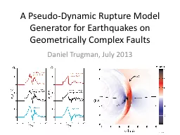
Daniel Trugman July 2013 2D RoughFault Dynamic Simulations Homogenous background stress complex fault geometry heterogeneity in tractions Eliminates important source of uncertainty fault geometry is a direct observable ID: 294636
Download Presentation The PPT/PDF document "A Pseudo-Dynamic Rupture Model Generator..." is the property of its rightful owner. Permission is granted to download and print the materials on this web site for personal, non-commercial use only, and to display it on your personal computer provided you do not modify the materials and that you retain all copyright notices contained in the materials. By downloading content from our website, you accept the terms of this agreement.
Slide1
A Pseudo-Dynamic Rupture Model Generator for Earthquakes on Geometrically Complex Faults
Daniel Trugman, July 2013Slide2
2D Rough-Fault Dynamic Simulations
Homogenous background stress + complex fault geometry
heterogeneity in tractionsEliminates important source of uncertainty: fault geometry is a direct observableSlide3
Rough Fault (not to scale)Slide4
“Pseudo-Dynamic” Source Model
Rough-fault simulations: high-frequency motions consistent with field observations
But: too computationally intensive to incorporate into probabilistic hazard analysisIdea: use insight from rough-fault simulations to build a “pseudo-dynamic
” source model
Source parameters consistent with dynamic models
Retain computational efficiency of kinematic modelsSlide5
Method:Building a Pseudo-Dynamic Model
Step 1: Study dynamic source parameters
Step 2: Represent pseudo-dynamic source parameters as spatial random fields that are consistent with dynamic simulationsStep 3: Compare source models and simulated ground motion for different fault profilesSlide6
Step 1: Analyze Dynamic
Source ParametersΔ
u, vrup
,
V
peak
Mean, standard deviations
Autocorrelation: spatial coherence
Dependence on fault geometry
Shape of source-time function,
V
(
t
)
R
estrict attention to:
subshear
ruptures (background stress just high enough for self-sustaining ruptures)
region away from the hypocenter (nucleation zone)Slide7
Source parameters are strongly
anti-correlated with fault slope
m
(
x
):Slide8
Source-time function of the form:Slide9
Step 2: Represent pseudo-dynamic source parameters as spatial random fields:
Assume Gaussian
marginalsUse mean, standard deviations from dynamic simulationsKey step:
anticorrelate
with fault slope
Assume
exponential ACF
:
Correlation length
β
from dynamic
sims
V
peak
,
Δ
u
more spatially
coherent than
v
rup
Power
spectrum ~
k
-2Slide10
Basic rupture generating procedure:Slide11
Step 3: Model Comparison
Start with a direct comparison on a single (random)
fractally-rough fault profileSource parameters and seismic wave excitationAlso compare with flat-fault projection of pseudo-dynamic source parameters
Generalize
to
ensemble comparison
30 different (random)
fractally
-rough fault profilesSlide12
final slip
, Δ
ucorrelation coefficient: 0.80
rupture velocity,
v
rup
correlation coefficient:
0.64
peak slip velocity,
V
peak
correlation coefficient:
0.78
Source ParametersSlide13
fault-parallel velocity (
v
x
)
fault-normal velocity (
v
y
)
SeismogramsSlide14
dynamic simulation
pseudo-dynamic simulation
Seismic
Wavefield
(fault-normal velocity)Slide15
rough fault
pseudo-dynamic simulation
flat fault
pseudo-dynamic simulation
Seismic
Wavefield
(fault-normal velocity)Slide16
Ensemble Marginal Distributions:Δ
u Slide17
Ensemble Marginal Distributions:
vrup Slide18
Fourier Amplitude Spectra
(fault-normal acceleration)Slide19
Peak Ground AccelerationSlide20
Discussion: generalization to 3D
2D autocorrelation structure i.e
βx
and
β
z
Which slope to use?
Trace of the fault plane in the slip direction?
Component of rupture velocity in
z
direction?
No correlation with
z
-direction slope (given stress field)?
Need to taper source parameter distributions at source boundaries?
Thrust faults?
Which is the relevant slope?
Is this different for rupture velocity than for slip?Slide21Slide22
Extra Slides:Slide23
Conclusions
Fault geometry strongly influences rupture process and hence, the earthquake source parameters.Our pseudo-dynamic model produces comparable ground motion to that seen in dynamic models, even at high frequencies.Similar models could be implemented in programs like
CyberShake to improve our understanding of seismic hazard.Slide24
Figure References
Dunham, E.M., Belanger, D., Cong, L., and J.E. Kozdon (2011). Earthquake ruptures with strongly rate-weakening friction and off-fault plasticity, Part 2:
Nonplanar faults, BSSA,
101
, no. 5, 2308-2322,
doi
: 10.1785/0120100076.
Graves, R. et al. (2011).
CyberShake
: A physics-based seismic hazard model for southern California
, Pure Appl.
Geophys
.,
168
, no. 3-4, 367-381,
doi
: 10.1007/s00024-010-0161-6.
Sagy
,
A.,Brodsky
, E. E., and G. J.
Axen
(2007). Evolution of fault-surface roughness with slip,
Geology
,
35
, 283-286,
doi: 10.1130/G23235A.1Shi, Z., and S. M. Day (2013). Rupture dynamics and ground motion from 3-D rough-fault simulations, J.
Geophys
. Res
. (in press).
Song, S. G. and L. A.
Dalguer
(2013). Importance of 1-point statistics in earthquake source
modelling
for ground motion simulation,
Geophys
., J. Int.
,
192
, no.3, 1255-1270,
doi
: 10.1093/gji/ggs089Slide25
Ensemble Marginal Distributions:
Vpeak Slide26
Peak Ground VelocitySlide27
Fourier Amplitude SpectraSlide28
Basic Procedure:
Generate fault profile h(x) (filter Gaussian noise in Fourier domain to obtain correct PSD)
Correlate source parameter vectors with m(
x
)
Filter correlated vectors to achieve desired PSD
Rescale and shift: correct mean and std. dev.
Aggregate source parameters
V
(
x,t
) Slide29
Complex Fault Geometry
Most dynamic rupture simulations assume planar faults, model stress field as random fieldBut faults are
fractally rough: deviate from planarity at all length scales:
Sagy
et
al.
Geology
2007
; 35: 283
-286
Dixie Valley Fault, Nevada