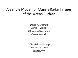
PPT-A Simple Model for Marine Radar Images of the Ocean Surface PowerPoint Presentation

David R Lyzenga David T Walker SRI International Inc Ann Arbor MI SOMaR3 Workshop July 1416 2015 Seattle WA Bragg Scattering According to the smallperturbation

Upload by giovanna-bartolotta
Published on 2015-11-09

Presentation Embed Code

<iframe width="560" height="315" src="https://www.docslides.com/embed/188299" frameborder="0" allowfullscreen></iframe>

Download Presentation

Download Presentation The PPT/PDF document "A Simple Model for Marine Radar Images o..." is the property of its rightful owner. Permission is granted to download and print the materials on this web site for personal, non-commercial use only, and to display it on your personal computer provided you do not modify the materials and that you retain all copyright notices contained in the materials. By downloading content from our website, you accept the terms of this agreement.