A study of the AMV correlation surface - PowerPoint Presentation

Slide1

A study of the AMV correlation surface

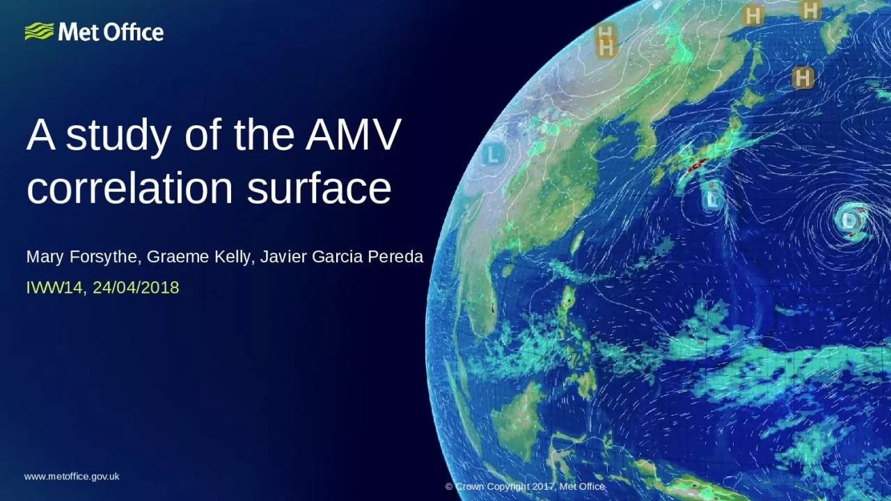
Mary Forsythe, Graeme Kelly, Javier Garcia PeredaIWW14, 24/04/2018

www.metoffice.gov.uk © Crown Copyright 2017, Met Office

© Crown copyright Met Office

Talk Outline

Motivation

Polar data

High resolution data

Global data

Early examples

How

can we use

the

information?

Motivation

T

T + 15

min

Infrared Imagery

Target Box / Tracer

e.g. 24 x 24 pixels

pixel – 3 km

Search Area

80 x 80 pixels centred on target box

3. Assign a

height

to the derived vector – moving towards use of optimal estimation - not always easy!

Initial corrections (image navigation etc.)

Tracking

How are AMVs produced?

Normally repeat from image 2-> 3 to give a second vector for quality control

new location determined by best match of individual pixel counts of target with all possible locations of target in search area.

For traditional AMV production from geostationary satellites - height assignment thought to be the dominant source of error – less focus given to tracking step.

But….

In recent years……

Greg Dew’s talk IWW10 Feb 2010

First challenge - polar winds

Image interval longer at ~100 min

Target size 28x28

Lots of noise in vector field due to longer image interval

Conclude: need first guess to guide tracking for polar winds

Kazuki

Shimoji’s

talk IWW12 Jun 2014

Second challenge – high resolution winds

Aim to generate winds more representative of local flow - move to smaller target box sizes

Target size 5x5

More noise, multiple peaks in correlation surface

NWP SAF – 4

th

analysis report – James Cotton, 2010

Third challenge – smoother cloud features

Example in jet region

1) 22 June 2) 29 June

Feature exhibiting large slow bias

Narrow jet core

Smooth linear features aligned parallel to direction of wind

Feature with fairly neutral bias

Much wider

Less regular - more contrast details perpendicular to flow

Differences

in texture of the two features may be affecting success of tracking

step.

Mean MetO background

O-B speed bias

Early examples

Plotting the correlation surfaces

Javier Garcia Pereda provided a modified

version of HRW v2016 (applicable with

NWCSAF v2016 only) which

includes the correlation matrices for each

AMV.

This is running in test mode at the Met Office and Graeme Kelly has put together some code to plot the correlation matrices for winds within the UKV domain.

Low level examples

At low level generally see cleaner correlation surfaces.

Correlation surface better constrained in area with more cloud texture

High level examples

At higher level – correlation surfaces can look quite messy!

How can we use the information?

Filtering to remove the poorly constrained cases

If correlation outside of a set region around the maximum correlation value exceeds a fraction of the maximum correlation – this test should remove cases with multiple maxima or broad maxima

Estimating tracking errors

Could attempt to fit an ellipse to the peak correlation structure – could provide estimates of error across both axes of the ellipse

NWP AMV observation error schemes

Several NWP centres use an observation error scheme based on the following assumption

Two

independent

sources of error

Error in vector

Linked to accuracy of tracking step

Error in height

Linked to accuracy of height assignment

More problematic if large vertical wind shear

A

good specification of the observation error is essential to assimilate in a near-optimal way

Total u/v error =

√ (

u/v Error

2

+

Error in u/v due to error in height

2

)

For this we need an estimate of:

u and v error (Eu

and Ev)

height error (Ep)

Potentially use information from the correlation surface for

Eu and Ev

See Forsythe & Saunders, IWW9, 2008 for more information

Summary

For many global AMVs – height assignment remains the main source of error

For polar AMVs and high resolution AMVs, the tracking step has proved more problematic due to longer image intervals (polar) or smaller target sizes (high resolution).

There may also be cases where traditional AMVs struggle due to smoother cloud features – in these cases motion often better constrained in one dimension.

There is information in the correlation surfaces that could be used to filter out poorly constrained cases or provide estimates of errors in the tracking step for use in NWP.

Next steps

So far the results have not shown much correlation between poorly constrained correlation surfaces and O-B fit, but we also haven’t seen cases where the AMVs look noisy.

We plan to look at reducing the quality control which might be filtering out the cases of poor tracking. We also plan to look at using smaller target box sizes which we know is more challenging.

We can then look again at whether there is a relationship with O-B fit.

Beyond that can we develop the ideas to provide flags or error estimates?

Spare slides

© Crown copyright Met Office

Mean MetO 250 hPa analysis wind speed

Meteosat-7 WV Indian Ocean – large slow bias feature

Persist May-Sept (SH Winter)

Example for June 2009

Closely matches location of sub-tropical Jet around 20-30S

Example 3

High level Jet region slow bias

O-B speed bias June 2009

Feature varies throughout June but not always coinciding with fastest wind speeds e.g.

Mean MetO background

O-B speed bias

© Crown copyright Met Office

Example 3High level Jet region slow bias

Case Study 1) 22 June 2009, 00UTC

Both sub-tropical Jet and Polar Jet show fast model wind speeds (>70 m/s) for AMVs (WV) associated with large slow biases

Slow bias

O-B speed bias

Jets

MetO model background wind speed

© Crown copyright Met Office

Example 3High level Jet region slow bias

Case Study 2) 29 June 2009, 00UTC

Jet to SE Madagascar shows fast wind speeds, but AMVs in this case with neutral (or even slightly fast) bias.

O-B speed bias

Jet

MetO model background wind speed

Why large slow biases associated with very fast winds in some cases and not others?