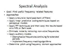
Spectral Analysis Goal: Find useful frequency related features - PowerPoint Presentation

Slide1

Spectral Analysis

Goal: Find useful frequency related features

Approaches

Apply a recursive band pass bank of filters

Apply linear predictive coding techniques based on perceptual models

Apply FFT techniques and then warp the results based on a MEL or Bark scale

Eliminate noise by removing non-voice frequencies

Apply auditory models

Deemphasize frequencies continuing for extended periods

Implement frequency masking algorithms

Determine pitch using frequency domain approachesSlide2

Cepstrum

History

(Bogert et. Al. 1963)

Definition

Fourier Transform (or Discrete Cosine Transform) of the log of the magnitude (absolute value) of a Fourier Transform

Concept

Treats the frequency as a “

time domain

” signal and computes the frequency spectrum of the spectrum

Pitch Algorithm

Vocal track excitation (E) and harmonics (H) are multiplicative, not additive. F1, F2, … are integer multiples of F0

The log converts the multiplicity to a sum

log(|X(

ω

)|) = Log(|E(

ω

)||H(

ω

)|) = log(|E(

ω

)|)+log(|H(

ω

)|)

The pitch shows up as a spike in the lower part of the CepstrumSlide3

Terminology

Cepstrum

Terminology

Frequency

Terminology

CepstrumSpectrumQuefrencyFrequencyRahmonicsHarmonicsGamnitudeMagnitudeSphePhaseLifterFilterShort-pass LifterLow-pass FilterLong-pass LifterHigh-pass-Filter

Notice the flipping of the letters – example

Ceps

is Spec backwardsSlide4

Cepstrum and PitchSlide5

Cepstrums for Formants

Time

Speech Signal

Frequency

Log Frequency

Time

Cepstrums of Excitation

After FFT

After log(FFT)

After inverse FFT of log

Answer:

It makes it easier to identify the formantsSlide6

Harmonic Product Spectrum

Concept

Speech consists of a series of spectrum peaks, at the fundamental frequency (F0), with the harmonics being multiples of this value

If we compress the spectrum a number of times (down sampling), and compare these with the original spectrum, the harmonic peaks align

When the various down sampled spectrums are multiplied together, a clear peak will occur at the fundamental frequency

Advantages: Computationally inexpensive and reasonably resistant to additive and multiplicative noiseDisadvantage: Resolution is only as good as the FFT length. A longer FFT length will slow down the algorithmSlide7

Harmonic Product Spectrum

Notice the alignment of the down sampled spectrumsSlide8

Frequency Warping

Audio signals cause cochlear fluid pressure variations that excite the basilar membrane. Therefore, the ear perceives sound non-linearly

Mel and Bark scale are formulas derived from many experiments that attempt to mimic human perceptionSlide9

Mel Frequency Cepstral Coefficients

Preemphasis

deemphasizes the low frequencies (similar to the effect of the basilar membrane)

Windowing

divides the signal into 20-30 ms frames with

≈50% overlap applying Hamming windows to eachFFT of length 256-512 is performed on each windowed audio frameMel-Scale Filtering results in 40 filter values per frameDiscrete Cosine Transform (DCT) further reduces the coefficients to 14 (or some other reasonable number)The resulting coefficients are statistically trained for ASRNote: DCT used because it is faster than FFT and we ignore the phaseSlide10

Front End Cepstrum ProcedureSlide11

Preemphasis/Framing/WindowingSlide12

Discrete Cosine Transform

Notes

N is the desired number of DCT coefficients

k is the “quefrency bin” to compute

Implemented with a double

for loop, but N is usually smallSlide13

MFCC Enhancements

Derivative and double derivative coefficients model changes in the speech between frames

Mean, Variance, and Skew normalize results for improved ASR performance

Resulting feature array size is 3 times the number of

Cepstral

coefficientsSlide14

Mean Normalization

public static double[][] meanNormalize(double[][] features, int feature)

{ double mean = 0;

for (int row: features)=0; row<features.length; row++)

{ mean += features[row][feature]; }

mean = mean / features.length; for (int row=0; row<features.length; row++) { features[row][feature] -= mean; } return features;} // end of meanNormalizeNormalize to the mean will be zeroSlide15

Variance Normalization

public static double[][] varNormalize(double[][] features, int feature)

{ double variance = 0;

for (int row=0; row<features.length; row++)

{ variance += features[row][feature] * features[row][feature]; } variance /= (features.length - 1); for (int row=0; row<features.length; row++) { if (variance!=0) features[row][feature] /= Math.sqrt(variance); } return features;} // End of varianceNormalize()Scale feature to [-1,1] - divide the feature's by the standard deviationSlide16

Skew Normalization

public static double[][] skewNormalize(double[][] features, int feature)

{

double fN=0, fPlus1=0, fMinus1=0, value, coefficient;

for (int row=0; row<features.length; row++) { fN += Math.pow(features[row][feature], 3); fPlus1 += Math.pow(features[row][feature], 4); fMinus1 += Math.pow(features[row][feature], 2); } if (momentNPlus1 != momentNMinus1) coefficient = -fN/(3*(fPlus1-fMinus1)); for (int row=0; row<features.length; row++) { value = features[row][column]; features[row][column] = coefficient * value * value + value - coefficient; } return features;} // End of skewNormalization()

Minimizes the skew for the distribution to be more normalSlide17

Mel Filter Bank

Gaussian filters (top), Triangular filters (bottom)

Frequencies in overlapped areas contribute to two filters

The lower frequencies are spaced more closely together to model human perception

The end of a filter is the mid point of the next

Warping formula: warp(f) = arctan|(1-a2) sin(f)/((1+a2) cos(f) + 2a) where -1<=a<=1|

Slide18

Mel Frequency TableSlide19

Mel Filter Bank

Multiply the power spectrum with each of the triangular Mel weighting filters and add the result -> Perform a weighted averaging procedure around the Mel frequencySlide20

Perceptual Linear Prediction

Cepstral Recursion

DFT of Hamming Windowed Frame

SpeechSlide21

Critical Band Analysis

The bark filter bank is a crude approximation of what is known about the shape of auditory filters.

It exploits Zwicker's (1970) proposal that the shape of auditory filters is nearly constant on the Bark scale.

The filter skirts are truncated at +- 40 dB

There typically are about 20-25 filters in the bank

Critical Band FormulasSlide22

Equal Loudness Pre-emphasis

private double equalLoudness(double freq)

{

double w = freq * 2 * Math.

PI;

double wSquared = w * w; double wFourth = Math.pow(w, 4); double numerator = (wSquared + 56.8e6) * wFourth; double denom = Math.pow((wSquared+6.3e6), 2)*(wSquared+0.38e9); return numerator / denom;}Formula (w^2+56.8e6)*w^4/{ (w^2+6.3e6)^2 * (w^2+0.38e9) * (w^6+9.58e26) }Where w = 2 * PI * frequencyNote: Done in frequency domain, not in the time domainSlide23

Intensity Loudness Conversion

Note:

The intensity loudness power law to bark filter outputs

which approximates simulates the non-linear relationship between sound intensity and perceived loudness.

private double[]

powerLaw(double[] spectrum) { for (int i = 0; i < spectrum.length; i++) { spectrum[i] = Math.pow(spectrum[i], 1.0 / 3.0); } return spectrum; }Slide24

Cepstral Recursion

public static double[] lpcToCepstral( int P, int C, double[] lpc, double gain)

{ double[] cepstral = new double[C];

cepstral[0] = (gain<

EPSELON) ? EPSELON : Math.log(gain);

for (int m=1; m<=P; m++) { if (m>=cepstral.length) break; cepstral[m] = lpc[m-1]; for (int k=1; k<m; k++) { cepstral[m] += k * cepstral[k] * lpc[m-k-1]; } cepstral[m] /= m; } for (int m=P+1; m<C; m++) { cepstral[m] = 0; for (int k=m-P; k<m; k++) { cepstral[m] += k * cepstral[k] * lpc[m-k-1]; } cepstral[m] /= m; } return cepstral;}

 Slide25

MFCC & LPC Based CoefficientsSlide26

Rasta (Relative Spectra) Perceptual Linear Prediction

Front EndSlide27

Additional Rasta Spectrum Filtering

Concept

: A b

and pass filters is applied to frequencies of adjacent frames. This eliminates slow changing, and fast changing spectral changes between frames. The goal is to improve noise robustness of

PLP

The formula below was suggested by Hermansky (1991). Other formulas have subsequently been tried with varying successSlide28

Comparison of Front End Approaches

Conclusion

: PLP and MFCC, and RASTA provide viable features for ASR front ends. ACORNS contains code to implement each of these algorithms. To date, there is no clear cut winner.