/
Use the Linear Approximation to estimate Use the Linear Approximation to estimate
Use the Linear Approximation to estimate - PowerPoint Presentation

mitsue-stanley
mitsue-stanley . @mitsue-stanley
Follow
393 views
Uploaded On 2017-12-17

Use the Linear Approximation to estimate - PPT Presentation

How accurate is your estimate Differential Notation The Linear Approximation to y f x is often written using the differentials dx and dy In this notation dx is used instead of ID: 616072

approximation error estimate linear error approximation linear estimate notation change tangent area graph small size tells

Share:

Link:

Embed:

Download Presentation from below link

Download Presentation The PPT/PDF document "Use the Linear Approximation to estimate" is the property of its rightful owner. Permission is granted to download and print the materials on this web site for personal, non-commercial use only, and to display it on your personal computer provided you do not modify the materials and that you retain all copyright notices contained in the materials. By downloading content from our website, you accept the terms of this agreement.


Presentation Transcript

Slide1
Slide2

Use the Linear Approximation to estimate

How accurate is your estimate?Slide3

Differential Notation

The Linear Approximation to

y

=

f

(x) is often written using the “differentials”

dx

and

dy

. In this notation,

dx

is used instead of

Δ

x to represent the change in x, and dy is the corresponding vertical change in the tangent line:

This is simply another way of writing

Δ

f

f

(a)Δ

x. Slide4

Differential Notation

How

much larger isSlide5

Thermal Expansion

A

thin metal cable has length

L

= 12 cm when the temperature is

T

= 21°C. Estimate the change in length when

T

rises to 24°C, assuming that

where

k

= 1.7 × 10

−5°C (k

is called the coefficient of thermal expansion).Slide6

Suppose that we measure the

diameter D

of a circle and use this result to compute the

area

of the circle. If our measurement of

D

is inexact, the area computation will also be inexact. What is the effect of the measurement error on the resulting area computation? This can be estimated using the Linear Approximation, as in the next example.Slide7

Effect

of an Inexact Measurement

The

Bonzo

Pizza Company claims that its pizzas are circular with diameter 50 cm

(a)

What is the area of the pizza?

(b)

Estimate the quantity of pizza lost or gained if the diameter is off by at most 1.2 cm.Slide8

Approximating

f(x)

by Linearization

If

f

is differentiable at

x = a

and

x

is closed to

a

, thenSlide9

Compute the linearization of at

a

= 1.Slide10

Estimate and compute the percentage error

.Slide11

The Size of the Error

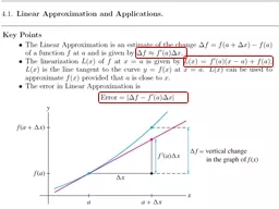
The examples in this section may have convinced you that the Linear Approximation yields a good approximation to

Δ

f

when Δx is small, but if we want to rely on the Linear Approximation, we need to know more about the size of the error:

Remember that the error E is simply the vertical gap between the graph and the tangent

line

.

where

K

is the maximum value

of |

f

(

x

)| on the interval from

a

to

a

+

Δ

x

. Slide12

The Size of the Error

The Error Bound tells us two important things. First, it says that the error is small when the second

derivative

(and hence

K

) is small. This makes sense, because

f

(

x

) measures how quickly the tangent lines change direction. When |

f

(

x

)| is smaller, the graph is flatter and the Linear Approximation is more accurate over a larger interval around

x

=

a

(compare the graphs). Slide13

The Size of the Error

Second, the Error Bound tells us that the error is of

order two

in

Δ

x

, meaning that

E

is no larger than a constant times (

Δ

x

)

2

. So if Δx is small, say Δx = 10−n, then E has substantially smaller order of magnitude (Δx)2 = 10−2

n. In particular, E/Δx tends to zero (because E/Δx <

KΔx), so the Error Bound tells us that the graph becomes nearly indistinguishable from its tangent line as we zoom in on the graph around x = a. This is a precise version of the “local linearity” property discussed in Section 3.2Slide14

4.1

SUMMARY

Let

Δ

f

=

f (a

+

Δ

x

) −

f (a)

. The

Linear Approximation

is the estimate

Differential notation:

dx

is the change in

x

,

dy

=

f

(

a

)dx

,

Δy

= f (a

+ dx

) − f

(a

). In this notation, the Linear Approximation reads

The

linearization

of

f

(

x

) at

x

=

a

is the function

The Linear Approximation is equivalent to the approximation

The error in the Linear Approximation is the quantity

In

many cases, the percentage error is more important than the error itself:Slide15