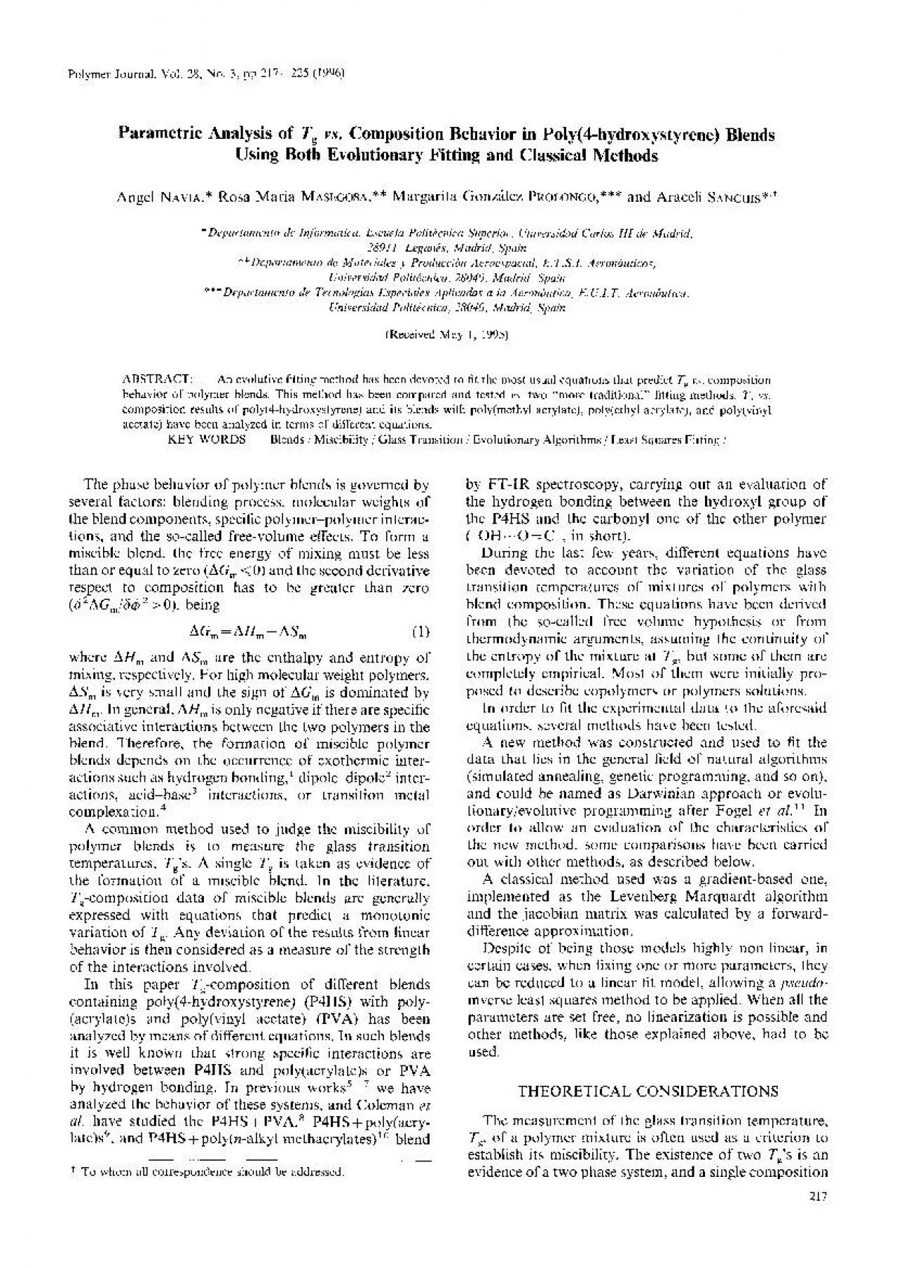
Polymer Journal Vol 28 No3 pp 217225 1996 Parametric Analysis of Tg v - PDF document

1 Polymer Journal, Vol. 28, No.3, pp 217-2
Polymer Journal, Vol. 28, No.3, pp 217-225 (1996) Parametric Analysis of Tg vs. Composition Behavior in Poly(4-hydroxystyrene) Blends Using Both Evolutionary Fitting and Classical Methods Angel NAVIA,* Rosa Maria MASEGOSA,** Margarita Gonzalez PROLONGo,*** and Araceli SANCHis*·t *Departamento de Informatica, Escuela Politecnica Superior, Universidad Carlos III de Madrid, 28911, Leganes, Madrid, Spain **Departamento de Materia/es y Produccibn Aeroespacial, E.T.S.l. Aeronauticos, Universidad Politecnica, 28040, Madrid, Spain ***Departamento de Tecnologias Especiales Aplicadas a Ia Aeronautica, E.U./.T. Aeronautica, Universidad Politecnica, Madrid, Spain (Received May I, 1995) ABSTRACT: An evolutive fitting method has been devoted to fit the most usual equations that predict T, vs. composition behavior of polymer blends. This method has been compared and tested vs. two "more traditional" fitting methods. T, vs. composition results of poly(4-hydroxystyrene) and its blends with poly( methyl acrylate), poly( ethyl acrylate), and poly( vinyl acetate) have been analyzed in terms of different equations. KEY WORDS Blends I Miscibility I Glass Transition I Evolutionary Algorithms I 1 The phase behavior of polymer blends is governed by several factors: blending process, molecular weights of the blend components, specific polymer-polymer interac­tions, and the so-called free-volume effects. To form a miscible blend, the free energy of mixing must be less than or equal to zero (t1Gm :S 0) and the second derivative respect to composition has to be greater than zero (b2L1Gm/bcp2�0), being (1) where L1Hm and t1Sm are the enthalpy and entropy of mixing, respectively. For high molecular weight polymers, t1Sm is very small and the sign of t1Gm is dominated by L1Hm. In general, L1Hm is only negative if there are specific associative interactions between the two polymers in the blend. Therefore, the formation of miscible polymer blends depends on the occurrence of exothermic inter­actions such as hydrogen bonding, 1 dipole-dipole2 inter­actions, acid-base3 interactions, or transition metal complexation.4 A common method used to judge the miscibility of polymer blends is to measure the glass transition temperatures, Tg's. A single Tg is taken as evidence of the formation of a miscible blend. In the literature, Tg-composition data of miscible blends are generally expressed with equations that predict a monotonic (P4HS) with poly­(acrylate)s and poly( vinyl acetate) (PV A) has been analyzed by means of different equations. In such blends it is well known that strong specific interactions are involved between P4HS and poly(acrylate)s or PV A by hydrogen bonding. In previous works5 -? we have analyzed the behavior of these systems, and Coleman et al. have studied the P4HS+PVA,8 P4HS+poly(acry­late)s9, and P4HS+poly(n-alkyl methacrylates)10 P4HS and the carbonyl one of the other polymer (-OH .. ·0 = C-, in short). During the last few years, different equations have been devoted to account the variation of the glass transition temperatures of mixtures of polymers with blend composition. These equations have been derived from the so-called free volume hypothesis or from thermodynamic arguments, assuming the continuity of the entropy of the mixture at Tg, but some of them are completely empirical. Most of them were a!Y In order to allow an evaluation of the characteristics of the new method, some comparisons have been carried out with other methods, as described below. A classical method used was a gradient-based one, implemented as the Levenberg-Marquardt algorithm and the jacobian matrix TIONS The measurement of the glass transition temperature, Tg, of a polymer mixture is often used as a criterion to establish its miscibility. The existence of two Tg's is an evidence of a two phase system, and a single composition 217 A. NAVIA eta/. dependent Tg is often taken as evidence of the formation of a miscible

2 blend. Experimental studies on the compo
blend. Experimental studies on the composition dependence of the glass transition for a large number of miscible binary polymer blends show both negative and positive deviations from a simple weighted average, i.e., a rule of mixtures, of the two Tg's of the pure polymers. With the exception of Brekner12•13 and Kwei14•15 equations, the most frequently cited expressions: Taylor, 16 Fox/7 Couchman,18-22 etc., are only able to predict Tg-composition curves that exhibit negative deviation from the rule of mixtures prediction. Positive deviation of this rule occurs in systems with strong intermolecular interactions, and the failure of the predictions is due to the inability of these equations to account for strong interactions.23 Schneider's et a/.23 equation allows to predict positive deviations but has two fit parameters that can't be determined separately. Kwei's equation can describe both negative and positive deviation as well as S-shaped Tg vs. composition curves, and has two parameters, one of them (K) is the same as the Taylor16 parameter, and represents the differences be­tween the components of the blend; usually K is taken as the quotient of the calorific capacities of the two polymers (K=ACPjACP)' and the other one (q) takes into account the specific interactions responsible of the miscibility of the mixture. In any case, when the Tg vs. composition curve is S-shaped, Schneider's et a!. ex­pression provides better fit than Kwei's one, due to the introduction of a cubic term in addition to a quadratic one. The cubic expression developed by Schneider et a/.12·13 on the basis of regular solutions applied to polymer blends, with the form: Tg-Tg1=(l+K )r:P-(K +K )r:P2+K r:P3 (2) T -T 1 1 2 2 g2 gl where ¢ is the corrected weight fraction of the stiffer polymer (with the higher glass transition temperature, Tg,): ¢ = ___ Kw2 w1 +Kwz (3) and K, K1, and K2 are fit parameters. K is the Taylor parameter, K1 represents the differences between the shares of the interaction energies of hetero and homo-contacts to be overcome at Tg to allow the characteristic conformational mobilities in the polymer blend. In addition, it includes the energetic perturbations in the molecular surroundings of the binary contacts. K2 considers the differences between the energetic perturba­tions in the molecular surroundings of the binary con­tacts. These authors have also demonstrated that ex­pression 2 can be reduced to Taylor and Fox expressions 4 and 5. If K2 = 0, this equation is the Kaning's one, 25·26 it be­comes Kwei's equation 6 if q=K K1(Tg2- Tg)(w1 -Kw2)2, and if K1 =0 and K2=0 it becomes ex­pression 4, in which if K = TgjTgz• is the Fox expres­sion 5. These equations are: Taylor: This equation was proposed to predict 218 the Tg of random copolymers from the Tg of the pure homopolymers, assuming volumes additivity, which implies free volumes additivity in polymer blends. T = w1 Tg, -j- Kw2 Tgz g w1 + Kwz (4) where K is a parameter of the model and is related with the nature of polymers of the blend. In the simplest case is a ratio of the two Tg's, TgjTgz' being the Fox expression 5. Fox: This expression assumes a random mixing of the polymer segments in the blend. 1 w1 Wz -= Tg Tg, Tgz (5) where w; is the weight fraction of polymer i in the blend (w2 = l-w1, therefore) and Tg, Tg, are the glass transition temperatures of the pure polymer i and the mixture, respectively. This model implies random mixture at segmental level of components and is frequently con­sidered as representation of ideal behavior in miscible polymer mixtures; due to this, and deviation of the ex­perimental data from this theoretical prediction is taken as criterion of the interaction strength between the amorphous phase components of the mixture. Kwei: To take into account the specific interactions, Kwei14·15 added to equation, a qua­dratic term, similar to the Jenkel and Hensch27 model ( qw 1 w2), and the expression is: w 1

3 Tg, + Kw2 Tgz Tg= +qw1w2 wl +Kwz
Tg, + Kw2 Tgz Tg= +qw1w2 wl +Kwz (6) with two fitting parameters, q and K. K is the Taylor parameter, which considers the differences be­tween mixture components and q represents the specific interactions responsible of the miscibility of the blend. SOLUTIONS TO LINEAR/NONLINEAR REGRESSION PROBLEMS Several Tg vs. composition models have been put under test, and the resulting test cases are summarized below: • case 1: K wei's equation, with k = I and q as parameter. • case 2: Kwei's equation, with q and k as parameters. • case 3: Schneider's equation with k= Tg)Tgz and k1, k2 as parameters. • case 4: Schneider's equation with k, k1, and k2 as parameters. This case is valuable to test the proposed methods as it is a highly nonlinear model, nevertheless, it has no real physical sense since the value of k has to be equal to the quotient of Tg1 and Tg2•12•13 The following minimization methods have been tested with every test case (when applicable): 1. Darwinian or evolutive programming was used to carry out the parametric modelling, such that every individual is represented by a vector of parameters (i.e., (q, k) for case 2), and the survival score is a function of the associated square error in fitting the data. With this assumptions, populations evolve towards a solution which is optimal in a least squares sense. More detailed Po1ym. J., Vol. 28, No. 3, 1996 Analysis of Polymer Blends with Evolutivc Methods explanation can be found in section of EVOLU­ TIONARY PROGRAMMING. 2. The second method used is a nonlinear gradient based one and it uses a modification of the Levenberg­Marquardt algorithm, the jacobian matrix being calcu­lated by a forward-difference approximation. An initial estimation of the parameters is useful, nevertheless, in order to perform a "fair" composition with the evolutive method, said initial value was randomly chosen in the interval (- 1.0, 1.0) for every parameter. The routine that implements this method has been extracted from NETLIB, a very widespread mathematical database. 3. Linear least squares using transformed variables. It is worth noting that many nonlinear models that might seem highly nonlinear at first glance can be put into linear form and a least squares fitting can be used, al­though in a suboptimal way. 26•28 A model is said linear if it can be expressed as linear combination of parameters and data, i.e., (7) This way, as long as the relation between the x;'s and a;'s is linear, the model is said to be linear, even in the case that the regressors xi's are a nonlinear function of some other regressors. There are some limitations, though, because the least squares fitting of the trans­formed variables is no longer least squares when re­garding the original data. In this way, a sensitivity study has been carried out to show that for the equations involved, the approximation is a valid one, as can be checked with the experimental results. Another dis­advantage is that the maximum likelihood nature of the least squares fitting is lost, because the distributions of the transformed variables is no longer gaussian, in general. The aforesaid approximation can be applied to the models involved here, the K wei model 6 and Schneider formula 2 in cases 1 and 3, respectively. It can be easily verified that for the case k= 1 in Kwei's and k= TgjTg2 in Schneider's the systems are linear: Kwei: y=q x x, being y=(Tg-w1 Tg, -w2Tg) (8) Schneider: y = k1 x x1 + k2x2, being y=(Tg-Tg)/(Tg2- Tg)-cf; xl ��=(1-12)' Xz=(¢3-cf;z) (9) In such cases, a matrix solution is possible in form of pseudo-inverse formulation which effectively solves the problem in a least square sense and as shown thereafter, the results completely agree with those yielded by gradient and evolutive methods. The matrix expression of eq 7 is as follows: (10) In the above equation, y represents a column vector of output variables (one regressand in our case) and X a matrix with as many columns as regressors, cor­res

4 ponding every row in the mentioned matri
ponding every row in the mentioned matrices to a different experimental observation, f!:. is the vector of parameters and is an error vector which represents Polym. J., Vol. 28, No.3, 1996 the maladjustment of experimental data to the model proposed. The objective is to obtain a least squares solution, equivalent to the minimization of the energy of vector e, which can be expressed as follows, min Ia( (e?))=min =min Ia IIl::- Xf!:.ll2 =min \a[(l::-Xf!:.)T(l::-XY:.)] (II) which yields, (12) This expression corresponds to the Moore-Penrose pseudo-inverse solution which has proved to be optimal in the least square sense. 28 It is necessary to verify that the solution is a minimum and not a maximum or saddle point. The minimum condition holds if the columns of X are linearly independent, in that case, a corollary states that (XT X) is positive-definite, guaranteeing the existence of the inverse. In any case, some other techniques might be necessary to avoid ill-conditioning of (XT X), such as SVD or QR decomposition. In any case, the least squares fitting performed in the "linearized model" concerns only the modified quantities y, x1, x2 (shown in expression 8 and 9) and in general it is not guarantied that a true least squares criterion is applied to the original variables Tg, w1, w2. In any case, it is clear from the experimental results that the results are negligible when dealing with practical problems. Some further analysis has been carried out to show that such approximation has also some other properties: it is an unbiased estimator as well and has bounded sensitivity values. It is well known from least squares theory that the sensitivity S of the parameter against perturbations in the data is somehow proportional to the averaged squared error times the squared condition number associated with X, y · e: x kff:(X), being This condition number has shown to be small for the experimental data concerned here. This way we can have a measure of the sensitivity of q with respect to x in the Kwei case (of k1, k2 with respect to x1, x2 in the Schneider case). If we can show that perturbations in the variables Tg, w1, w2 are transmitted to x, x1, x2 without excessive amplification, we can assure that the method is valid, even being suboptimal. This can be checked with the partial derivatives of the expressions involved, with the result that all of them are bounded: Kwei: dy -·-=1· dT ' g dx --=1-2w1 dw1 Schneider: dx -=0· dT ' g (14) 219 A. NAVIA eta/. dy dx1 -=0· dT ' g dxz =0. dT ' g dy -K dx1 =(1-2¢) K dw1 [w1 +K(l-w1)]2 dxz =(3¢2-2¢) K 2 dw1 [w1 + K(1-w1)] (15) The sensitivity parameters have shown to be bounded and of similar magnitude for every experimental data set, being: Linearization in K wei model: k2(X) X Linearization in Schneider model: k2(X) X EVOLUTIONARY PROGRAMMING The adaptive algorithm proposed here to solve the curve fitting problem is evolutionary programming, which lies in the general field of natural algorithms. In 1958, Brooks35 described a creeping random method where k points were generated via gaussian perturbations about a search point. The best point was kept and the process repeated. Brooks observed that "there are some rather intriguing analogies that can be made between the creeping random method and evolution." Fogel et a/.11•33•36 proposed a similar scheme termed evolutiona­ry programming where, instead of keeping the best point, a population of search points is maintained. The underlying idea is that any animal species has to modify itself in order to cope with changes in environ­mental conditions or just to accomplish a better adapta­tion to its environment. This task is carried out by natural selection operating upon the individuals in the population. This way, only the fittest ones are ex­pected to survive and breed the next generation. The rules used to decide whether an individual is to survive or not are expressed in terms of a "fitness function," which depends on the s

5 pecific problem to solve. The general ev
pecific problem to solve. The general evolution of the population should therefore maximize that function by means of survival and breeding of the fittest individuals. 25•30·11 In our case, the problem could be outlined as follows: every individual has to represent by itself a valid solution to the problem, it might be built with the free parameters of the equations (e.g., individual= (K, K1, K2) for Schneider's eq 2). It is quite important to express an individual in a minimal form, this is, if there is any relation between any parameters, try to express one/ several of them as a function of the other and include only the latter into the individual (this makes the algorithm much more robust and faster as well). According to this, it is possible to assign a "fitness score" to every individual, which can be computed, in our case, as the mean squared error of the experimental data to the curve defined by the individual under 220 Rejected individuals Memory Search Ranked population Next generation do =0, Figure 1. Fogel original offspring rule. Rejected individuals Ranked population Memory Refining Close search Remote search Next generation O'o =0, O't Figure 2. Modified offspring rule. evaluation. Adaptation operates only through competi­tive selection among the individuals of a population and a subset of them is selected to produce the next generation. As can be observed in Figure l, Fogel11 proposed an offspring method in which half population is rejected and the rest is used to obtain the next gen­eration. This method has been refined and the pro­posed scheme is depicted in Figure 2. By all means, this method has to be much more effective than pure random search in order to be valuable, and indeed it is. A decisive factor is the kind of operations performed over the individuals, for instance, genetic algorithms generally use three kinds of operations: mutation, crossover, and inversion. It has been stated that crossover and inversion work well for small coding structures, but for large ones, they force evolution to approach a random search. The above mentioned operations are only a subset of all the possible ones and the applicability of each one of them is strongly problem dependent. In evolutionary programming, probabilistic survival is used instead by placing each member of the population in competition against some percentage of the other individuals and the probability of "winning" is related to their respective fitness. Offspring computa­tion is performed using gaussian mutations. A brief reminder of the algorithm is shown in Table V. A general comparison between genetic30•33 and evolutionary algorithms11 shows that the former certainly provides an initial search that is more efficient than random search but usually falls in sub optimal solutions while the latter is robust to multiple minima and can optimize functions of many variables which have nonlinear interactions. The gaussian relationship between parent and offspring guarantees that every point in the parameter space can be reached and the probabilistic survival allows every possible solution to be kept, avoiding premature convergence. Finally, if a parallel processing machine is available, the total computation time can be tremend­ously reduced because evolutionary algorithms can easily be executed in parallel machines. Polym. J., Vol. 28, No. 3, 1996 Analysis of Polymer Blends with Evolutive Methods EXPERIMENTAL CONSIDERATIONS Poly(4-hydroxystyrene) (P4HS), poly(vinyl acetate) (PVA), poly(methyl acrylate) (PMA), and poly(ethyl acrilate) (PEA) were purchased from Polysciences (U.K.). Two different samples of P4HS have been used, one of Mn=5100 and the other of Mn=1500 (HSVA15). Polymer characterization, blends preparation and differential scanning calorimetry (DSC) are detailed in previous works. 5•6 RESULTS AND DISCUSSION Schneider and coworkers have analyzed T -composi­tion behavior for some polymer blends. consider that segmental alignment due

6 to specific directed in­teractions betwe
to specific directed in­teractions between two different polymers lies to a re­duction in the free volume, causing a lowering in the mobility of the polymer blend. This lowering corre­sponds to a positive deviation from the rule of mixtures prediction for the Tg-composition behavior. In strongly auto associated polymers, association broken due to the second component of the mixture is a positive contribution to the free volume, opposite to the other, and Tg behavior in miscible blends will be a balance between both terms, finding both positive and negative deviations in Tg vs. composition Kwei's model: when K= 1, Kwei's equation becomes: Tg= [w1 Tg, +w2Tg,] +qw1w2, (12) where the term in brackets represents aditivity value and q is a parameter which is positive when, in average, the interactions between chains of the different polymers are stronger than those between chains of the same polymer, otherwise, q 0. In all the systems studied here, we have obtained q 0, which can be understood considering that miscibility process is a result of the equilibrium reached between the number of weak -OH···-C=O bonds formed and the number of stronger --OH · · · HO- broken. Since additivity law would correspond to a case in which the contact energies between polymers after blending are similar to contact energies in each homopolymer, q and therefore Tg (w1 Tg, + w2 Tg2) may be expected from the above discussion. Coleman eta!. 9 suggested that miscibility of blends of P4HS and poly(n-alkyl acrylate) decreased with increas­ing n as a result of the increasing steric difficulty for the formation of -OH···C=O bonds. This is in accordance with Tg vs. w behavior showed in Figures 4 and 6 for P4HS + PMA and P4HS +PEA, the opposite behavior than that of the absolute difference between Tg and the additive value of Tg and therefore of the q parameter. This is more evident for P4HS + PV A (Figures 2 and 5) systems where the lower fraction of hydroxyl groups involved OH···OH bonds the more negative is q and hence the larger is the difference between the experimental Tg and the additive value. Comparing Tg vs. w behavior of systems of P4HS of two different molecular weights with PV A, can be confirmed that the hydrogen bonding is more effective for the blends with P4HS of lower molecular weight. In Schneider's model, K, K1, and K2 are constants arising from the model, that in general are treated as adjustable parameters. According to the model, K1 is related to the differences between the interaction energies between contact sites in chains of the same kind and those in chains of different species. K2 reflects the perturbations in the interactions between sites arising 400 g 350 {! 300 0 0,1 0,2 0,3 0,4 0,5 0,6 0,7 0,8 0,9 W2 Figure 3. Kwei equation curve fitting for the P4HS+PMA and P4HS+PEA systems. 0. P4HS+PMA; ------,curve fitting; e. P4HS+PEA; -, curve fitting. Polym. J., Vol. 28, No.3, 1996 221 A. NAVIA eta/. 450r----------------------------------------------------------------------------------, ·· .. o 400 350 t- 300 0 0,1 0,2 0,3 0,4 0,5 0,6 0,7 0,8 0,9 W2 Figure 4. Kwei's equation curve fitting for P4HS+PVA and P4HS (JSOO)+PVA. e. P4HS(l500)+PVA; --.curve fitting; 0. P4HS+PVA; ------, curve fitting. 400 0 0,1 0,2 0,3 0,4 0,5 W2 0,6 0,7 0,8 0,9 Figure 5. Schneider's equation curve fitting for P4HS + PMA and P4HS +PEA systems. 0. P4HS + PMA; ------, curve fitting, e. P4HS + PEA; --, curve fitting. from the different molecular environments in which the sites may be. Finally K is a characteristic of the nature of the polymers and, in the simplest case, is related to a 222 ratio of the Tg's of the two homopolymers. The values obtained for K1 and K2 are similar to those obtained in the literature12·13 for systems with Tg vs. w behavior Polym. J., Vol. 28, No. 3, 1996 400 ;z Ci 350 1- 300 Analysis of Polymer Blends with Evolutive Methods 0 0,1

7 0,2 0,3 0,4 0,5 W2 0,6 0,7 0,8
0,2 0,3 0,4 0,5 W2 0,6 0,7 0,8 0,9 Figure 6. Schneider's equation curve fitting for P4HS+PVA and P4HS (1500)+PVA systems. e. P4HS (1500)+PVA; --,curve fitting; 0. P4HS +PYA; ------. curve fitting. HSVA HSEA HSMA HSI5VA Table I. Results of fitting' K wei equation (k =I, q free) Linearization Gradient q Av. err./K q Av. err./K -70.237 2.17 -70.2543 2.17 -7.966 4.84 -7.9678 4.84 -47.239 4.15 -47.254 4.15 -6.615 2.29 -6.617 2.29 Standard deviationsb: uq.GRAo=5.6£-3, uq,l!v=9.4E-4. Evolutionary q -70.237 -7.966 -47.241 -6.616 Av. err./K 2.17 4.84 4.15 2.29 "Every parameter shown in the tables has been presented with too many decimals, such a precision is only for comparison purpose and has got no physical sense, as the measurement errors are usually much more noticeable. b These are mean values of the standard deviation of every one of the four cases under test, such values have shown to be of the same order of magnitude and therefore presented as averaged. Table II. Results of fitting' Kwei equation (k and q both free) Gradient Evolutionary ------- ------- ----k q Av. err./K k q Av. err./K HSVA HSEA HSMA HSISVA 0.9825 0.991 0.9914 0.5944 -68.177 -6.489 -46.06 42.156 -----2.18 4.87 4.17 2.18 1.0 1.0 1.0 0.5976 -70.276 -8.0 -47.265 41.679 2.17 4.84 4.15 2.17 Standard deviationsh: uk.GRAo=0.0137, O'k.Ev=2.6£-4; uq,GRAo= 1.032, uq,Ev=0.047. ----- --· ---- -------- a Every parameter shown in the tables has been presented with too many decimals, such a precision is only for comparison purpose and has got no physical sense, as the measurement errors are usually much more noticeable. h These are mean values of the standard deviation of every one of the four cases under test, such values have shown to be of the same order of magnitude and therefore presented as averaged. similar to our systems. Characteristics of the Algorithm Presented Several fitting tests were performed over the available Polym. J., Vol. 28, No. 3, 1996 data obtained by direct measurements as previously mentioned. Every data set contained ten equally spaced data points and every fitting algorithm was executed ten times, yielding a set of model parameters than have 223 A. NAVIA et al. Table III. Results of fittinga Schneider's equation (k= T.,!T.,, k1, k2 free) --------kl HSVA -0.6164 HSEA 0.1844 HSMA -0.366 HSISV 0.333 Linearization Gradient --------kl Av. err./% kl kl Av. err.jK --------------------- -------- -0.714 0.0121 -0.6186 0.0119 -0.9132 0.0157 0.2971 0.0225 -0.616 0.1846 -0.365 0.3315 -0.713 -0.6184 -0.913 0.2937 0.0122 0.0119 0.0158 0.0225 -0.6162 0.1844 -0.365 0.333 Evolutionary k 2 -0.7136 -0.6188 -0.9135 0.2974 Av. err./K 0.0121 0.0119 0.0157 0.0225 --------- -------------- ----------- -------- Standard deviationsb: o-k,,GRAo= 1.1£-3, o-k,.Ev=7.5£-4; o-k,.GRAo= 1.8£-3, o-k,.Ev=6£-4. "Every parameter shown in the tables has been presented with too many decimals, such a precision is only for comparison purpose and has got to physical sense, as the measurement errors are usually much more noticeable. b These are mean values of the standard deviation of every one of the four cases under test, such values have shown to be of the same order of magnitude and therefore presented as averaged. Table IV. Results of fittinga Schneider's equation (k, and k2 free) ----- ----------- Gradient' Evolutionary k kl kl Av. err.jK k k1 k2 Av. err.jK ------- ·---- HSVA 0.9866 -0.8158 -0.4596 0.0115 0.9983 -0.821 -0.4458 0.0115 HSEA 0.8677 -0.3048 -0.831 0.01 0.8708 -0.3098 -0.8315 0.01 HSMA l.ll47 -0.8517 -0.771 0.0111 1.117 -0.853 -0.764 0.0111 HS15VA 0.3501 1.596 1.444 0.0177 0.348 1.607 1.4582 0.0177 "Every parameter shown in the tables has been presented with too many decimals, such a precision is only for comparison purpose and has got no physical sense, as the measurement errors are usually much more noticeable. b These are mean values of the standard deviat

8 ion of every one of the four cases under
ion of every one of the four cases under test, such values have shown to be of the same order of magnitude and therefore presented as averaged. 'Several epochs have not been used here, as the gradient algorithm shown to have some problems with local minima. Table V. The evolutionary algorithm I. Initialize the population randomly and compute the initial fitness F, of every individual P,. {P,}, i=l,N; F,=F(G(P;)) The functions F( · ) and G( · ) are highly dependent on the problem. 2. Modify every individual in the following way: P,: = P, + N(O, sF,+ Z) , where the operator ": =" denotes calculation for the next generation, s is a parameter that depends on the offspring rule used and N( · ) represents a normal function. 3. Compute the fitness of every new individual. F,=F(G(P;)) 4. Alternatively, some kind of probabilistic competition can be used: Compute for every individual the number of "wings" W, in the following way m i= I w,, t= 1 {1 if ul t= () 0 otherwise ul, u2 random (0, 1), r=int(Nxu2+1), "m" denotes the number of fights for every individual. 5. Rank the population using either the fitness score or the number of wins. 6. Go back to step 2 and repeat until convergence. --------------------been presented averaged and with standard deviation references. It is worth mentioning that the precision used when presenting the numbers in the tables is of little 224 practical meaning because the measurement errors are supposed to be at least one order of magnitude bigger than the precision shown; nevertheless they are useful to compare the performance and characteristics of the algorithms under test. Four different cases are presented. The Kwei equation with k equal to I and q free is the simplest model, it is linearizable in a straightforward way as shown before and represents a curve with no inflexion points (k = I). The results are shown in Table I. This model is not able to represent correctly the HS 15V A case. This case has got an inflexion point and, as shown in Table II, when letting the k parameter freely fluctuate, it converges to a value different of I (k � 0.6) and also produces a different value in q, thereby reducing the error. In both cases, the standard deviations of the evolutive method is one or several orders of magnitude smaller than the gradient method ones. In any case, the fitting errors shown in Table II are still too big, because the model lacks of enough degrees of freedom to cope with variations in the data. With the Breckner's equation, we are able to model the data with much lower fitting errors. The only case with real physical meaning is the one with k= Tg/Tg, although the case with k free has also been introduced to test the algorithms in a more difficult case, as the former is easily linearizable. Again, the standard deviations are much lower in the case of evolutive programming and parameters are more accurate, at the same time. It is important to note that when letting k, k1, and k2 free, the problem highly nonlinear and so, the gradient method proved to be highly dependent on the initialization, very often getting stuck on local minima, far from the optimal solution (see note 3). In this sense, the evolutionary algorithm has proved to be much more Polym. J., Vol. 28, No. 3, 1996 Analysis of Polymer Blends with Evolutive Methods robust against local mtmma, always converging to the global minimum. CONCLUSIONS AND FINAL REMARKS A new algorithm has been developed and tested in order to fit the parameters in every parametric model. The above detailed evolutionary algorithm has proved to be robust, accurate and easy to program, when compared to other techniques as those based on surface descent following the direction of the gradient. In general, the standard deviations of the fitting process for different epochs are smaller than with other methods (see Table I), allowing a small number of simulations to be carried out in order to find a good estimate of the correct values. The n

9 on-linearity of the equations involved s
on-linearity of the equations involved seems to represent no inconvenient for the optimum development of the search in the parameter space; the main limitation is that the speed of convergence becomes slow for high dimensional parameter spaces, due to the excessive number of degrees of freedom. Anyway, some further studies are being carried out to progress in that direction. In any case, we encourage people to use the evolutive method in cases with highly nonlinear interactions be­tween parameters and regressors in which the classical methods have shown lack of robustness. REFERENCES I. M. M. Coleman and P. C. Painter, Appl. Speclrosc. Rev., 20. 255 (1984). 2. E. M. Woo, J. W. Barlow, and D. R. Paul, J. Appl. Polym. Sci., 28, 1347 (1983). 3. Z. L. Zhow and A. Eisemberg, J. Polym. Sci., Polym. Leu. Ed., 21, 233 (1983). 4. A. Sen and R. A. Weiss, Polym. Prepr., Am. Chem. Soc., Div. Polym. Chem., 28 (2), 220 (1987). 5. A. Sanchis, R. M. Masegosa, R. G. Rubio, and M.G. Prolongo, Eur. Polym. J., 30, 781 (1994). 6. A. Sanchis, M.G. Prolongo, R. G. Rubio, and R. M. Masegosa, Polym. J., I, 10 (1995). 7. A. Sanchis, M.G. Prolongo, R. M. Masegosa, and R. G. Rubio, Macromolecules, 28, 2693 (1995). 8. E. J. Moskala, S. E. Howe, P. C. Painter, and M. M. Coleman, Macromolecules, 17, 1671 (1984). Polym. J., Vol. 28, No. 3, 1996 9. M. M. Coleman, A. M. Lichkus, and P. C. Painter, Macro­molecules, 22, 586 ( 1989). 10. C. J. Scrman, P. C. Painter. and M. M. Coleman, Polymer, 32, 1049 (1991). 11. D. V. Fogel, "'System Identification through Simulated Evolution: A Machine Learning Approach to Modeling," GINN Press, Aylesbury, Great Britain, U. K .. 1991. 12. M. J. Brcckner, H. A. Schneider, and H. J. Cantow, Polymer, 29, 78 ( 1988). 13. M. J. Breckner, H. A. Schneider, and H. J. Cantow, Makromol. Chem., 189, 2085 (1988). 14. T. K. Kwei, J. Polym. Sci., Polvm. Lett. Ed., 22, 308 (1962). I 5. A. A. Lin, T. K. Kwci, and A. Reiser, Macromolecules, 22, 4112 (1989). 16. M. Gordon and J. S. Taylor, J. Appl. Chem., 2, 493 (1952). 17. T. G. Fox, Proc. Am. Phys. Soc., l, 123 (1956). 18. P.R. Couchman, Macromolecules, 11, 1156 (1978). 19. P.R. Couchman, Phys. Lett., 70A, 155 (1979). 20. P. R. Couchman, J. Appl. Phys., 50, 6043 ( 1979). 21. P. R. Couchman and F. E. Karasz, Macromolecules, II, 117 (1978). 22. P.R. Couchman, J. Mater. Sci., 15, 1680 (1980). 23. J. M. Rodrigucz-Parada and V. Perec, Macromolecules, 22, 4112 (1989). 24. M. Vivas de Meftahy and J. M. J. Frechet, Polymer, 29, 447 (1988). 25. G. Kaning, Kolloid Z.-Z. Polym., 190, 1 (1963). 26. G. Kaning, Kolloid Z.-Z. Polym., 223, 54 (1969). 27. E. Jenckel and R. Heusch, Kolloid Z.-Z. Polym., 130, 89 (1953). 28. J. H. Holland, "Adaptation in Natural and Artificial Systems," MIT Press, Bradford Books edition, Michigan, MI, 1975. 29. H. Bunke and 0. Bunke, "'Nonlinear Regression, Functional Relations and Robust Methods," John Wiley & Sons, New York, N.Y., 1989. 30. D. M. Bates, "Nonlinear Regression Analysis and Its Applications," John Wiley & Sons, New York, N.Y., 1989. 31. D. Cuthbert and F. S. Wood, "Fitting Equations to Data: Computer Analysis of Multifactor Data," John Wiley & Sons, New York, N.Y .. 1980. 32. D. S. Borowiak, "'Model Dicrimination for Nonlinear Regression Models," Marcel Dekker, New York, N.Y., 1989. 33. D. E. Goldberg, "Genetic Algorithms in Search, Optimization and Machine Learning," Addison-Wesley, New York, N.Y., 1989. 34. D. Docampo and A. Navia, "Solving Iterated Function Systems using Evolutionary Algorithms," COST Second Vigo Workshop on Adaptive Methods and Emergent Techniques for Signal Processing and Communications, Vigo, Spain, June 1993. 35. L. Brooks, "A Discussion of Random Methods for Seeking Maxima," Operations Research, 6, 244 (1958). 36. D. B. Fogel, IEEE Journal on Oceanic Eng., 17, 333 (19