PPT-Designing Effective Monitoring Programs for Fish Population Response to Habitat Restoration

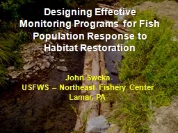
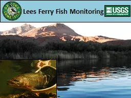
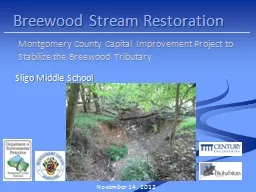
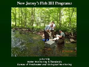
John Sweka USFWS Northeast Fishery Center Lamar PA What is the goal of fish habitat restoration efforts and partnerships To create morebetter fish habitat To enhancerecoverrestore fish populations. Christian . Knoth. , . Birte. Klein, . Till . Kleinebecker. , . Torsten. . Prinz. , Birgit . Sieg. Ifgicopter. Group – University of Muenster. Joint Meeting of Society of Wetland Scientists, . Wetpol. Lees Ferry Monitoring. Annual sampling. Electrofishing. Abundance, Size. Angler Surveys. Catch rates. How do Glen Canyon Dam operations influence the rainbow trout fishery?. Modified low fluctuating flows. STILL . MAY NOT COME. Using new knowledge to move beyond physical restoration of wildlife habitat. Conservation Biology Research Group. Prof Michael . Mahony. , Dr John . Clulow. and . Alexandra Callen. By . Professor Olanrewaju .A. Fagbohun, . Ph.D. Nigerian Institute of Advanced Legal Studies. University of Lagos Campus. Akoka, Lagos. Presentation made at the International Conference on . Oil and Gas Dispute Resolution . Montgomery County Capital Improvement Project to. Stabilize the Breewood Tributary. November 14, 2012. Sligo Middle School. Introductions. . Doug Marshall. Watershed Planner, Montgomery County Department of Environmental Protection (MCDEP). Fish Oil Market Report published by value market research, it provides a comprehensive market analysis which includes market size, share, value, growth, trends during forecast period 2019-2025 along with strategic development of the key player with their market share. Further, the market has been bifurcated into sub-segments with regional and country market with in-depth analysis. View More @ https://www.valuemarketresearch.com/report/fish-oil-market Lees Ferry Monitoring. Annual sampling. Electrofishing. Abundance, Size. Angler Surveys. Catch rates. How do Glen Canyon Dam operations influence the rainbow trout fishery?. Modified low fluctuating flows. John Vile Water Monitoring & Standards Bureau of Freshwater and Biological Monitoring What is a Fish Index of Biotic Integrity? 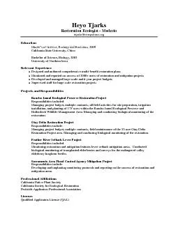Using fish assemblages to assess the overall health of a stream ecosyst Restoration Ecologist - Modesto htjarks@riverpartners.org Education Master’s of Science, Ecology and Evolution, 2009 California State University, Chico Bachelor of Science, Biology, 2003 University [DOWNLOAD] Préparer et réussir le Bac Pro ELEEC - T1 Habitat individuel, locaux industriels et habitat tertiair: T1 Habitat individuel, locaux industriels et habitat tertiaire
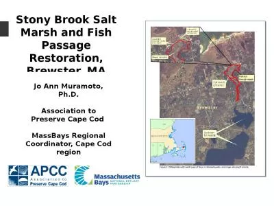
http://skymetrix.xyz/?book=2100576321 the Carolina Vegetation Survey . Protocol. M. Forbes Boyle, Robert K. Peet, Thomas R. Wentworth, and Michael Lee. 17 November 2010. The CVS Team. Project Directors. Robert Peet, UNC Chapel Hill. Thomas Wentworth, NC State University. . Jo Ann . Muramoto. , Ph.D.. Association to Preserve Cape Cod . MassBays. Regional Coordinator, Cape Cod region. . Problems. Salt marsh was degraded by insufficient tidal flow due to an undersized 4’ culvert under a state highway;. Lots of dishes and meals can be made with fish.. Fish dishes. Name this fish dish.. Have you tried this before?. Fish fingers, chips and peas. Fish dishes. Name this fish dish.. Which country does this dish come from?. How are these fish different?. Fish. What do you notice about each of these fish?. How many types of fish can you name?. Name this fish. Prawn. Name this fish. Mackerel. Name this fish. Haddock. Name this fish.