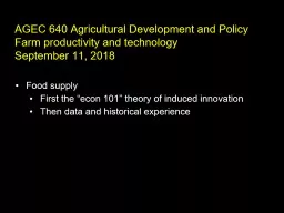
Farm productivity and technology September 11 2018 Food supply First the econ 101 theory of induced innovation Then data and historical experience Lets start with a conclusion ID: 748803
Download Presentation The PPT/PDF document "AGEC 640 Agricultural Development and ..." is the property of its rightful owner. Permission is granted to download and print the materials on this web site for personal, non-commercial use only, and to display it on your personal computer provided you do not modify the materials and that you retain all copyright notices contained in the materials. By downloading content from our website, you accept the terms of this agreement.
Slide1
AGEC 640 Agricultural Development and PolicyFarm productivity and technologySeptember 11, 2018
Food
supply
First the “econ 101” theory of induced innovation
Then data and
historical
experienceSlide2
Let’s start with a conclusion…From Econ 101: Innovation is only path to sustained growthSwitch from self-sufficiency to markets gives (big?) one-time gainOnce in markets, better prices give further (small?) one-time gains...with diminishing marginal physical products!New technologies that raise physical productivity are essential
Higher average product boosts payoff with same inputs
Higher marginal product induces investment in more
inputs
Let’s build the analysis, piece by piece
…Slide3
To explain production and technology choices…
Qty. of corn
(bu/acre)
Qty. of beans
(bushels/acre)
observed production
(whatever it is)
observed consumption
(production +/- transactions)
observed transactions
(purchase, sale, gifts etc.)Slide4
To explain production and technology choices, we start with a household model
Qty. of corn
(bu/acre)
Qty. of beans
(bushels/acre)
other possible buy/sell choices
(the “income” line)
slope is -
Pb
/Pc
(price of beans /
price of corn)
observed production
(whatever it is)
observed consumption
(production +/- transactions)
other possible choices
(the “production possibilities frontier”)
In economics, each observed choice is already an optimum… for the chooser!
observed transactions
(purchase, sale, gifts etc.)
other equally preferred choices (consumers are already at highest
level of “utility” they can reachSlide5
Decisions on input use can be understood in a similar way:
Qty. of corn
(bu/acre)
Qty. of labor
(hours/acre)
Qty. of machinery
(hp/acre)
Qty. of labor
(hours/acre)
highest profits
(slope=Pl/Pc
)
lowest cost
(slope=-Pl/Pm)
observed input use
(whatever it is)
other possible choices
“input supply curve”
“isoquant”
(each curve shows
other possibilities
if nothing else changes
)
What does the observed input use optimize?
Here, production choices depend only on market prices; when all inputs and outputs can be bought/sold, production is “separable” from consumptionSlide6
…here is the complete picture:
Qty. of corn
(bu/acre)
Qty. of labor
(hours/acre)
Qty. of corn
(bu/acre)
Qty. of beans
(bushels/acre)
Qty. of machinery
(hp/acre)
Qty. of labor
(hours/acre)
profits
(slope=Pl/Pc
)
income
(-Pb/Pc)
cost
(slope=-Pl/Pm)
Now… if the individual is already optimizing,
how can their productivity and well-being ever improve?
utilitySlide7
Productivity can improve through the market,from self-sufficiency to specialization
Qty. of corn
(bu/acre)
Qty. of beans
(bushels/acre)
If beans are more valuable in the market than on the farm…
self-sufficiency
(production= consumption)
adjusting production
to market prices can overcome diminishing returns on the farm
production was chosen along PPF, to highest indifference curve
from consumption
…trading allows the farmer to reach whatever consumption gives a higher utility levelSlide8
Once people are already trading in the market,if prices “improve” production will rise
Qty. of corn
(bu/acre)
Qty. of labor
(hours/acre)
Qty. of corn
(bu/acre)
Qty. of beans
(bushels/acre)
Qty. of machinery
(hp/acre)
Qty. of labor
(hours/acre)
Price of inputs falls, relative to output
Price of goods sold rises, relative to purchased goods
Price of labor rises, relative to cost of labor-saving technologies
…but with diminishing returns,
productivity
must fall,
with less and less output per unit of input.Slide9
How can productivity rise?when people are already doing the best they can,…and are facing diminishing returns? Slide10
Productivity growth requires innovation:a change in what is physically possible
Qty. of corn
(bu/acre)
Qty. of labor
(hours/acre)
Qty. of corn
(bu/acre)
Qty. of beans
(bushels/acre)
Qty. of machinery
(hp/acre)
Qty. of labor
(hours/acre)
more of both outputs for given resources
less of both inputs needed for given outputs
more output at each input levelSlide11
Two prominent innovations
Ag. output
(tons/hectare)
Qty. of fertilizer
(tons/hectare)
Qty. of labor
(days/hectare)
Qty. of traction
(hp/hectare)
Hybrid corn
Herbicide-Tolerant
SeedsSlide12
The price ratio is the same. How does the new technology affect input use?
Ag. output
(tons/hectare)
Qty. of fertilizer
(tons/hectare)
Qty. of labor
(days/hectare)
Qty. of traction
(hp/hectare)
IRC w/new hybrid
IRC w/old variety
Isoquant w/old tech.
Isoquant w/new seeds
optimum with old variety
optim.w/old tech.Slide13
Is it still optimal to use the old input levels?
Ag. output
(tons/hectare)
old qty. of fertilizer
Qty. of labor
(days/hectare)
IRC w/new
IRC w/old
Isoquant w/old
Isoquant w/new
old tractor setSlide14
Ag. output
(tons/hectare)
old qty. of fertilizer
Qty. of labor
(days/hectare)
IRC w/new
IRC w/old
Isoquant w/old
Isoquant w/new
old tractor set
In these cases, farmers can (and will?) adopt these new technologies at the old input levels…Slide15
This innovation is profitable and cost-reducing, without changing input levels
more output
same qty. of fertilizer
Qty. of labor
(days/hectare)
IRC w/new
IRC w/old
Isoquant w/old
Isoquant w/new
same tractor set
higher
profit
lower
costs
less labor
Ag. output
(tons/hectare)Slide16
But adjusting input use to the new technologyis even better (higher profits, lower costs)
even more output
more fertilizer
Qty. of labor
(days/hectare)
Ag. output
(tons/hectare)
highest-possible profit along the IRC w/ new hybrids
more
labor
less
horsepower
lowest-possible cost along the isoquant w/ new herbicidesSlide17
The change in marginal products determines farmers’ incentives to change input levels
Ag. output
(tons/hectare)
Qty. of fertilizer
(tons/hectare)
Qty. of labor
(days/hectare)
Qty. of traction
(hp/hectare)
When the input response curve gets
steeper,
farmers are induced to use more fertilizer and increase output
When the isoquant gets
flatter
, farmers are induced to use more labor and less horsepowerSlide18
New techniques using less horsepower
Can this type of thinking help us predict what types of new technology are most desirable?
Ag. output
(tons/hectare)
Qty. of fertilizer
(tons/hectare)
Qty. of labor
(days/hectare)
Qty. of traction
(hp/hectare)
New techniques using fewer workers
New techniques using
more fertilizer
than currently
being used
New techniques
using less fertilizerSlide19
New techniques are most desirable if they help farmers use the abundant factor. This is known as “induced innovation”.Ag. output(tons/hectare)labor-using, yield-increasing innovations
labor-saving,
yield-increasing
innovations
Qty. of
labor
(tons/hectare)
new
old
Qty. of
labor
(tons/hectare)
new
oldSlide20
Some conclusions…From Econ 101: Innovation is only path to sustained growthSwitch from self-sufficiency to markets gives (big?) one-time gainOnce in markets, better prices give further (small?) one-time gains...with diminishing marginal physical products!New technologies that raise physical productivity are essential
Higher average product boosts payoff with same inputs
Higher marginal product induces investment in more
inputs
But, there is a bit more to the story…Slide21
In the US… abundant cropland, expanding until 1935; so farm machinery spread early in 19th century, and little yield or productivity growth until 1930sIn Japan… scarce cropland, with widespread irrigation so fertilizer and new seeds spread early in 19th century, and little machinery use or labor saving until 1960s
The Hayami & Ruttan (1985) example:
Farm technology in U.S. and Japan, 1880-1980Slide22
Slide 22Japan’s rollout of new rice varieties began in 1880sSlide23
Slide 23US spread of hybrid corn occurred later,in S-shaped adoption curves with varied start dates, speed of diffusion and ceiling levelSlide24
The “induced innovation” idea also applies across farms within a country, as we saw here… Slide25
The green revolution uses international R&Dto spread crop improvement faster• In 1920s, an early green revolution occurred in E. Asia, as Japan bred new rice for their colonies in Taiwan & Korea.• After WWII, threat of mass starvation and communism led U.S. and others to improve wheat for S.Asia & S.America, and new rice varieties for South & Southeast Asia.• In recent years, some (smaller) effort to do this for AfricaSlide26
Key characteristics of “green revolution” technologyshort stature, toconcentrate nutrients in grain, not stalk, andsupport more grain without falling over (lodging);photoperiod insensitivity, togive flexibility in planting/harvest dates, control maturation speed, with more time for grain filling, and
early maturity for short rains or multicropping
many other traits
pest and stress resistance
leaf structure and positionSlide27
The speed and timing of the green revolutionvaries by regionReproduced from W.A. Masters (2008), “Beyond the Food Crisis: Trade, Aid and Innovation in African Agriculture.” African Technology Development Forum 5(1): 3-15.
US, Europe starts pre-WWII
East Asia starts post-WWII
S. & SE Asia starts in late 1960s
Africa’s slow and delayed green revolution has barely started!Slide28
Selected Soil Fertility Constraints in Agriculture(as percent of agricultural area)Note: Constraints characterized using the Fertility Capability Classification (Sanchez et al., Smith).Source: Stanley Wood (2002), IFPRI file data.
Why are Africa’s yield gains slow & delayed?
One reason is soils and moistureSlide29
Source: Calculated from data in Evenson and Gollin, 2003.But crucially, most African farmers still use old seed types; new seeds are coming out nowSlide30
Source: Calculated from IFPRI and FAOStat file dataA key reason for delayed adoption is less local research to meet local needs
Public Research Expenditure per Unit of Land, 1971-91
(1985 PPP dollars per hectare of agricultural land)
0
1
2
3
4
1971
1972
1973
1974
1975
1976
1977
1978
1979
1980
1981
1982
1983
1984
1985
1986
1987
1988
1989
1990
1991
Sub-Saharan Africa
All Developing Countries
All Developed CountriesSlide31
The composition of foreign aid to Africa has changed radically over timeReproduced from W.A. Masters (2008), “Beyond the Food Crisis: Trade, Aid and Innovation in African Agriculture.” African Technology Development Forum 5(1): 3-15.
In the 1970s and 1980s, donors gave much more food aid than aid for agricultural production
In the 1990s and 2000s, health and debt relief grew; food aid declined but so did aid for agricultureSlide32
Why has there been so little efforton food crop improvement for Africa?Early conditions were unfavorableUntil early 1960salmost all of Africa was under European colonial rule most countries were land-abundant exporters of cash cropsUntil mid-1980smost African governments taxed agriculture heavily, asthe region remained land abundant (but exported less and less)
When population growth finally outstripped land supply in the 1980s and 1990s, the rest of the world…
was awash in grain – no fear of mass starvation
had won cold war – no fear of Africa becoming communist
seen export growth in Asia – thought Africa could import its foodSlide33
To respond to farmers’ needs, crop improvement involves multiple innovationsGenetic improvement
(by scientists, using controlled trials)
Agronomic improvement
(by farmers, using land & labor)Slide34
Slide 34New techniques to manage soils and conserve moisture are spreading
traditional
“flat” planting
labor-intensive
“Zai” microcatchments
For these fields, the workers are:Slide35
The role of policy in agricultural technologyInnovation is subject to severe market failuresR&D + dissemination is often…a natural monopoly“non-rival” in production, with high fixed costs, low or zero marginal costa provider of public goods“non-excludable” in consumption, so difficult or impossible to recover costsR&D activity often involves asymmetric informationa “credence good” for investors in R&D and for potential adopters of new technologies
Thus private firms provide too little innovation…
the pace and type of innovation depends crucially on government, using its monopoly of force and taxation.Slide36
How can government lead society to do more innovation?public research and education from 1100s in Europe, rise of Medieval universities from 1870s in US and Japan, founding of agricultural researchpatents in 1624, Britain enacted a formal “Statute of Monopolies”; in 1787, patent law written into Article 1 of the U.S. constitutionprizes in 1714, the British Parliament offered a £20,000 reward for an accurate way to measure longitude at sea many other examples…Policy options to promote innovationSlide37
Is there enough R&D?Economists suspect under-spending, perhaps because:benefits are dispersed and hard to observe, and costs are specific and easy to observemost analysis try to answer using returns to research:if returns are above average, there is under-spending;if returns are below average, there is over-spending.What do Alston et al. find?confirms systematic under-spending (high returns),but finds large variance in results, possibly due to: poor measurementvariance in the management of research inherent riskiness of research activitiesSlide38
Slide 38Slide39
What’s new in ag. research?Reproduced from Clive James (2008), Global Status of Commercialized Biotech/GM Crops: 2008. ISAAA Brief No. 39. ISAAA: Ithaca, NY (www.isaaa.org).Global Area of Biotech Crops, 1996 to 2008:Industrial and Developing Countries (m. ha)
Indust. Co.
:
5.4% of
1.29 b. ha
Worldwide
: 2.5% of
4.96 b. ha
Dev’ing. Co.
:
1.5% of
3.67 b. ha
Approx. share of global farm area in 2008
Molecular biology!Slide40
New biotechnologies hold great promisebut so far only for a few cropsReproduced from Clive James (2008), Global Status of Commercialized Biotech/GM Crops: 2008. ISAAA Brief No. 39. ISAAA: Ithaca, NY (www.isaaa.org).Global Area of Biotech Crops, 1996 to 2008,By Crop (millions of hectares)
Maize
:
24% of 157 m. ha
Soybeans
: 70% of
95 m. ha
Canola
:
20% of 30 m. ha
Cotton
:
46% of 34 m. ha
Share of global area for that crop in 2008Slide41
New biotechnologies hold great promisebut so far only through a few traitsReproduced from Clive James (2008), Global Status of Commercialized Biotech/GM Crops: 2008. ISAAA Brief No. 39. ISAAA: Ithaca, NY (www.isaaa.org).Global Area of Biotech Crops, 1996 to 2008,By Trait (millions of hectares)Slide42
Reproduced from Clive James (2008), Global Status of Commercialized Biotech/GM Crops: 2008. ISAAA Brief No. 39. ISAAA: Ithaca, NY (www.isaaa.org).USA 62.5 m.
Mexico 0.1 m.
Honduras <0.05 m.
Colombia
<0.05 m.
Bolivia 0.6 m.
Chile <0.05 m.
Argentina 21 m.
Uruguay 0.7 m.
Paraguay 2.7 m.
Brazil 15.8 m.
S.Africa 1.8 m.
Australia 0.2 m.
Burkina Faso <0.05 m.
Philippines 0.4 m.
India
7.6 m.
China 3.8 m.
Egypt
<0.05 m.
Romania <0.05 m.
Slovakia <0.05 m.
Poland
<0.05 m.
Czech R.
<0.05 m.
Germany
<0.05 m.
Spain 0.1 m.
Portugal
<0.05 m.
Canada
7.6 m.
Global Status of Biotech/GM Crops (hectares in 2008)
New biotechnologies hold great promise
but so far a relatively narrow impact
only
cotton
mainly
cottonSlide43
Some more conclusions…In practice: Innovation sometimes responds to incentives
“Induced” innovation would save increasingly scarce resources, and use increasingly abundant ones
But public action is needed to drive and direct technology
Patents and other IPRs where copying is easily detected
Public investment where gains are non-excludable
(as in much of agricultural research!)