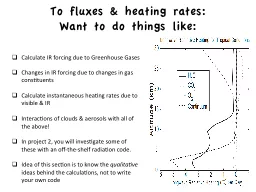
Want to do things like Calculate IR forcing due to Greenhouse Gases Changes in IR forcing due to changes in gas constituents Calculate instantaneous heating rates due to visible amp IR Interactions of clouds amp aerosols with all of the above ID: 542489
Download Presentation The PPT/PDF document "To fluxes & heating rates:" is the property of its rightful owner. Permission is granted to download and print the materials on this web site for personal, non-commercial use only, and to display it on your personal computer provided you do not modify the materials and that you retain all copyright notices contained in the materials. By downloading content from our website, you accept the terms of this agreement.
Slide1
To fluxes & heating rates:Want to do things like:
Calculate IR forcing due to Greenhouse GasesChanges in IR forcing due to changes in gas constituentsCalculate instantaneous heating rates due to visible & IRInteractions of clouds & aerosols with all of the above!In project 2, you will investigate some of these with an off-the-shelf radiation code.Idea of this section is to know the qualitative ideas behind the calculations, not to write your own codeSlide2
Monochromatic Intensity (nonscattering) at wavenumber
Intensities (up and down) anywhere in atmosphere
Transmittance between layer z1 and z2
Optical depth
btn
z1 & z2
Contribution from each layer z’ to the intensity at z goes like this.
Must sum over all LINES and continuum contribution to get full absorption coefficient at Slide3
Must take into account contributions from potentially many gas absorption lines.Multiple calculations to get all layers in atmosphere. But is easily do-able.
To integrate over real instrument response functions, may have to average over several closely-spaced values.Monochromatic Intensity (nonscattering) at wavenumber Slide4
Monochromatic Fluxes?
Can do angular integral by replacing B with πB, and t(z1,z2) with tF(z1,z2), which is the monochromatic “flux transmittance”. Showed in book that can get away with “2-stream approximation”: where =~ 3/5, or θ ~ 53° Slide5
Broadband fluxes?
Needed to calculate forcings (ie cloud forcing, greenhouse gas forcing)Needed to calculate heating ratesThus, needed in all weather and climate models!Must integrate over all wavelengths!! 350 cm-1
670 cm
-1
1250 cm
-1
5000 cm
-1Slide6
How many wavelengths do we need for the broadband calculation?
In infrared, need typically 20 to 2000 cm-1. Scales of vibrational “bands” (e.g. CO2 ν2) is 10s of cm-1 wide. Can roughly approximate Planck function as constant across this scale.Scales of rotational line spacing is ~ 1 cm-1.Scales of rotational line widths (needed to resolve lines: ~ 10-2 (near surface) to 10-4 cm-1 (in stratosphere).Slide7
Line-by-line: The accurate but REALLY slow method
With a modest spacing of 0.001 cm-1, need ~ 2106 monochromatic RT calculations (assuming 2 stream) just to do IR at one model grid point.Models may have 104-106 grid points.Calculation must be done every time step (multiple times per day, perhaps every 1-3 hrs
).
Much too slow for weather/climate models, but can use it for limited testing and validation (e.g. LBLRTM)
LW or SWSlide8
Monochromatic Flux Reminder
where:Flux Weighting Function
Monochromatic Flux TransmittanceSlide9
Another way forward: spectral bands
Write as flux contributions from many spectral intervals
Assume
P
lanck B is constant over each spectral interval
Band-averaged transmittance over spectral intervalSlide10
Molecular
SpectroscopyAbsorption Lines;absorption coefficientpressure & temperature dependence
Transmission properties of
a single line @
fixed p &T
Broadband transmission at
fixed p &T
Empirical -band
absorption as a
func.
of
path
K-distribution
bin by strength
Band models
statistical treat-
ment
of lines,
distribution of
strengths and
centers
Line-by-line
direct sum over
all lines, direct
integration over
frequency and
path
Transmission
models
Integral over many lines
Integral over single line
TOPICS
The absorption path length
(mass path)
Theory of absorption/transmission by
a single
line
(NOT
TERRIBLY USEFUL)
Spectrally integrated over bands of overlapping lines
Empirical
Band models
K-distribution Slide11
Gas
Path
/ Absorber Mass Path
Mass mixing
ratio
Units are kg/m
2
. Slide12
Two versions
of
mass
path
k constant (horizontal)
k changing (vertical)
k changes in the vertical due only do changes in line widths (which depend on P and T) and line strengths (which depend on T)
Mass abs.
coeff
:
m
2
/ kg of gas
Absorber mass path:
kg/m
2
of gas
Gas
Path
/ Absorber Mass PathSlide13
1
0
transmission
W(u)
Theory
of Frequency-Integrated Absorption by a Single Line
In this theory, absorption is typically expressed as an equivalent width (units of frequency, wavenumber, wavelength) and is the absorption by an equivalent, hypothetical square opaque lineSlide14
1
0
transmission
W(u)
Theory of Frequency-Integrated Absorption by a Single Line
The equivalent width
W(u)
u
Curve
of growth
Assumes a uniform path
(
ie
non varying P & T)
ΔνSlide15
Frequency-Integrated Absorptionby a Single Line (contd)
Two basic limits (for convenience set
0
=0)
:
1. Weak line limit (linear)
ie W(u) is linear in uSlide16
Frequency-Integrated Absorptionby a Single Line (contd)
2. Strong line limit (square root)
Consider the line
wings of a pressure-broadened line
ie W(u) is goes as sqrt in uSlide17
Frequency-Integrated Absorptionby a Single Line (summary)
Curve of growth
Weak line limit occurs as line centers fill in (u small)
Strong line limit occurs as wings broaden out (u big)Slide18
The
Empirical Approach to
Broadband
Absorption
favored before the advent of computing power and availability
of spectroscopic data bases – also favored approach of GCM model Parameterizations in 70s & 80s – also useful for estimating bulk solar absorption
Examples of empirical broad-band relations
Provided the absorptions are (spectrally)
independent
Slide19
Typical values of
column ozone - 300 DU~
0.3 cm NTP)
Example#1 of the UV broad-band curve of growthSlide20
Band Models
Treat spectral interval as containing either regularly spaced or randomly occurring linesTypically assume homogeneous P & T (like on a horizontal path) – no pressure broadening! Later on relax this with additional approaches.Not always very accurate (not using real spectroscopy! Essentially fit 2 parameters to spectroscopy)Slide21
Band Models
Equally spaced lines by δLines all have same strength S
y=α
L
/
δ
is the “grayness parameter”
Randomly spaced lines, average line spacing is
δ
Lines have distribution of strengths:
Malkmus
ModelSlide22Slide23
Malkmus
Band
model: Parameter fits
For different bands, you run a line-by-line reference code and fit parameters to the transmittance as a function of u.
Parameters for the Random/
Malkmus
model shown (taken from Stephens notes)Slide24
Inhomogenous
Paths – HCG Approximation(van de Hulst – Curtis – Godson)p2p
1Slide25
k
k
j
-dk/2
k
j
+dk/2
The
k-Distribution
Method – more modern approach
f(
k
j
) is the fraction of the interval
where
k
j
-dk
/2<k
<
k
j
+dk
/2Slide26
Vs. Frequency
Sorted lowest-to-highestInhomogenous Paths – “Correlated-K method”Slide27
Vs. Frequency
Sorted lowest-to-highestInhomogenous Paths – “Correlated-K method”Slide28Slide29
Local Heating Rate – depends on the rate of change of the net flux
because an increase in Fnet(z) with increasing z implies a cooling.
Note the sign convention Petty uses!Slide30
Flux equations (SW or LW!)
Band-averaged transmittance over spectral interval
Recall Band-Averaged TransmittanceSlide31
Difference to get NET Flux at level z
Could combine, but we will leave separate!
Now just differentiate
w.r.t
. z…Slide32
D
ifferentiate w.r.t. z to get Heating Rate due to spectral band ΔνiSlide33
Heating Rate due to spectral band
Δνi (Form 1)Flux from surface
Flux from TOA
Flux from layers below
Flux from layers above
Emission Downwards
Emission DownwardsSlide34
Heating Rate due to spectral band
Δνi (Form 2)Coupling with Surface
Coupling with Space
(
LW: Cooling
;
SW: Heating
)
Coupling with layers above
Coupling with layers belowSlide35
Fluxes & heating ratesSlide36
Shortwave Heating
Terms C+D = 0 because there is no Shortwave emission in atmosphere.Term (B) dominates (absorption from TOA).H2O & Ozone are the dominant gases. Their density profiles, SZA and clouds determine the heating rate profilesH2O dominates in troposphere; Ozone dominates in stratosphere.Slide37
Heating rates decline when sun is lower in sky!
Implies a strong diurnal and seasonal cycle.Slide38
Longwave Heating&Cooling
Depends upon both gas profiles AND temperature profileTerm (B) dominates: “Cooling-to-Space approximation”H2O, CO2 dominant; Ozone important in stratosphere.CO2 has mild heating right at tropopause; strong cooling above as “cooling-to-space” term kicks in.H2O Dominant in lower atmosphere; two peaks due to two absorption features (18-25 micron pure rotation feature & 5-8 micron vibration feature)Slide39
From BUGSrad! Tropical atmosphere
In stratosphere, LW & SW nearly balance (over a full diurnal cycle!)In troposphere, other heating terms from sensible & Latent heating balance the stronger LW cooling.Can easily see the little “CO2 Peak” at the tropopauseSlide40
Project 2Use Online tool to explore LW & SW heating rates and effects due to adding clouds & gases.
Write-up to explain what you found.