/
Quantile plots:  New  planks in an old campaign Quantile plots:  New  planks in an old campaign

Quantile plots: New planks in an old campaign - PowerPoint Presentation

phoenixbristle
phoenixbristle . @phoenixbristle
Follow
342 views
Uploaded On 2020-08-28

Quantile plots: New planks in an old campaign - PPT Presentation

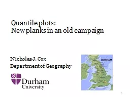
Nicholas J Cox Department of Geography 1 Quantile plots Quantile plots show ordered values raw data estimates residuals whatever against rank or cumulative probability or a onetoone function of ID: 809381

quantile plots values data plots quantile data values plot box stata distributions journal letter command probability axis normal plotting

Share:

Link:

Embed:

Download Presentation from below link

Download The PPT/PDF document "Quantile plots: New planks in an old c..." is the property of its rightful owner. Permission is granted to download and print the materials on this web site for personal, non-commercial use only, and to display it on your personal computer provided you do not modify the materials and that you retain all copyright notices contained in the materials. By downloading content from our website, you accept the terms of this agreement.


Presentation Transcript

Slide1

Quantile plots: New planks in an old campaign

Nicholas J. CoxDepartment of Geography

1

Slide2

Quantile plots

Quantile plots show ordered values (raw data, estimates, residuals, whatever)

against rank or cumulative probability or a one-to-one function of the same.

Tied values are assigned distinct ranks or probabilities.

2

Slide3

Example with auto dataset

3

Slide4

quantile default

In this default from the official command quantile, ordered values are plotted on the

y axis and the fraction of the data (cumulative probability) on the x axis. Quantiles (order statistics) are plotted against plotting position (

i − 0.5)/n for rank i

and sample size

n

.

Syntax was

sysuse

auto, clear

quantile mpg, aspect(1)

4

Slide5

Quantile plots have a long history

Adolphe

Quetelet

Sir Francis Galton G.

Udny

Yule Sir Ronald Fisher

1796–1874 1822–1911 1871–1951 1890–1962

all used quantile plots

avant

la

lettre

.

In geomorphology, hypsometric curves for showing altitude distributions are a long-established device with the same flavour.

5

Slide6

Quantile plots named as such

Martin B. Wilk Ramanathan

Gnanadesikan 1922–2013 1932–2015Wilk, M. B.

and Gnanadesikan, R. 1968.

Probability plotting methods

for the

analysis

of

data.


Biometrika


55: 1–17.

6

Slide7

A relatively long history in Stata

Stata/Graphics User's Guide (August 1985) included do-files quantile.do and

qqplot.do. Graph.Kit (February 1986) included commands

quantile, qqplot

and

qnorm

.

Thanks to Pat

Branton

of StataCorp for this history.

7

Slide8

Related plots use the same information

Cumulative distribution plots show cumulative probability on the y axis. Survival function plots show the complementary probability.

Clearly, axes can be exchanged or reflected. distplot (Stata Journal ) supports both.

Many people will already know about sts

graph

.

8

Slide9

So, why any fuss?

The presentation is built on a long-considered view that quantile plots are the best single plot for univariate distributions. No other kind of plot shows

so many features so well across a range of sample sizes with so few arbitrary decisions.Example: Histograms require binning choices. Example: Density plots require kernel choices. Example: Box plots often leave out too much.

9

Slide10

What’s in a name? QQ-plots

Talk of quantile-quantile (Q-Q or QQ-) plots is also common. As discussed here, all quantile plots are also QQ-plots.

The default quantile plot is just a plot of values against the quantiles of a standard uniform or rectangular distribution. 10

Slide11

NJC commands

The main commands I have introduced in this territory are quantil2

(Stata Technical Bulletin) qplot

(Stata Journal)

stripplot

(SSC)

Others will be mentioned later.

11

Slide12

quantil2

This command published in Stata Technical Bulletin 51

: 16–18 (1999) generalized quantile:One or more variables may be plotted.

Sort

order may be

reversed.

by()

option is supported.

Plotting

position

is generalised to

(

i −

a

) /(

n

− 2

a

+ 1): compare a = 0.5 or (i − 0.5)/n wired into quantile. 12

Slide13

qplot

The command quantil2 was renamed qplot

and further revised in Stata Journal 5: 442−460 and 471 (2005), with later updates: over() option is also supported.

Ranks may be plotted as well as plotting positions.

The

x

axis scale may be transformed on the fly.

recast()

to other

twoway

types is supported.

13

Slide14

stripplot

The command stripplot

on SSC started under Stata 6 as onewayplot in 1999 as an alternative to graph, oneway

and has morphed into (roughly) a superset of the official command dotplot

.

It is mentioned here because of its general support for quantile plots as one style and its specific support for quantile-box plots, on which more shortly.

14

Slide15

Comparing two groups is basic

superimposedjuxtaposed

15

Slide16

Syntax was

qplot mpg, over(foreign) aspect(1)

stripplot mpg, over(foreign) cumulative centre vertical aspect(1

)

16

Slide17

Quantiles and transformations commute

In essence, transformed quantiles and quantiles of transformed data are one and the same, with easy exceptions such as reciprocals reversing order. So, quantile plots mesh easily with transformations, such as thinking on logarithmic scale.

For the latter, we just add simple syntax such as ysc(log).

Note that this is not true of (e.g.) histograms, box plots or density plots, which need re-drawing.

17

Slide18

The shift is multiplicative, not additive?

18

Slide19

A more unusual example

Glacier terminus position change may be positive or negative, with possible outliers of either sign. Cube root transformation pulls in both tails and (fortuitously but fortunately) can separate advancing and retreating glaciers.

Here we use the stripplot command and data from Miles, B.W.J., Stokes, C.R., Vieli, A. and Cox, N.J. 2013. Rapid, climate-driven changes in outlet glaciers on the Pacific coast of East Antarctica. Nature 500:

 563–566.

19

Slide20

20

Slide21

21

Slide22

multqplot (Stata Journal)

multqplot

is a convenience command to plot several quantile plots at once. It has uses in data screening and reporting. It might prove more illuminating than the tables of descriptive statistics ritual in various professions.

We use here the Chapman data from Dixon, W. J. and

Massey,

F.J. 1983

.

Introduction to Statistical Analysis

.

4th

ed

. New

York: McGraw–Hill.

22

Slide23

23

Slide24

multqplot defaults

By default the minimum, lower quartile, median, upper quartile and maximum are labelled on the y axis

– so we are half-way to showing a box plot too. By default also variable labels (or names) appear at the top.

More at Stata Journal 12:549–561 (2012) and 13:640–666 (2013).

24

Slide25

multqplot

choicesNaturally we can reach through to use options of

qplot and graph twoway.

Here we use normal quantile plots.

The normal (Gaussian) can serve as a reference distribution even if we have good grounds for doubting that it will be observed.

25

Slide26

26

Slide27

Raw or smoothed?

Quantile plots show the data as they come: we get to see outliers, grouping, gaps and other quirks of the data, as well as location, scale and general shape. But sometimes the details are just noise or fine structure we do not care about. Once you register that values of

mpg in the auto data are all reported as integers, you want to set that aside. You can smooth quantiles, notably using the Harrell and Davis method, which turns out to be bootstrapping in disguise. hdquantile

(SSC) offers the calculation.

27

Slide28

Harrell, F.E. and Davis,

C.E. 1982. A new distribution-free quantile estimator. Biometrika 69: 635–640.

28

Slide29

Letter values

Often we do not really need all the quantiles, especially if the sample size is large. We could just use the letter values, which are the median, quartiles (fourths), octiles (eighths), and so forth out to the extremes, halving the tail probabilities at each step.

lv supports letter value displays. lvalues is now available to generate variables.

See Stata Journal 16:1058–1071 (2016

).

Thanks to David

Hoaglin

for suggesting use of letter values at the 2016 Chicago meeting.

29

Slide30

Parsimony of letter values

For n data values, there are 1 + 2 ceil(log2 n

) letter values . For n = 1000, 106 , 10

9, there are 21, 41, 61 letter values.

We will see examples shortly.

30

Slide31

Fitting or testing named distributions

Using quantile plots to compare data with named distributions is common. We had an example earlier.

The leading example is using the normal (Gaussian) as reference distribution. Indeed, many statistical people first meet quantile plots as such normal probability plots. It seems that these were first used in 1894 by

Pierre Jean Paul Henry (1848–1907),

who

taught

artillery

at Fontainebleau.

http://serge.mehl.free.fr/chrono/Henry.html

31

Slide32

Pawitan’s principle

Yudi Pawitan in his 2001 book In All Likelihood (Oxford University Press) advocates normal QQ-plots as making sense generally — even when comparison with normal distributions is not the goal.

32

Slide33

qnorm available but limited

qnorm

is already available as an official command — but it is limited to the plotting of just one set of values.

33

Slide34

Named distributions with qplot

qplot has a general

trscale() option to transform the x axis scale that otherwise would show plotting positions or ranks. For normal distributions, the syntax is just to add

trscale

(

invnormal

(@))

@

is a placeholder for what would otherwise be plotted.

invnormal

()

is Stata’s name for the normal quantile function (as an inverse cumulative distribution function).

34

Slide35

35

Slide36

A standard plot in support of t tests?

This plot is suggested as a standard for two-group comparisons:We see all the data, including outliers or other problems.

Use of a normal probability scale shows how far that assumption (read: ideal condition) is satisfied. The vertical position of each group tells us about location, specifically means.

The slope or tilt of each group tells us about scale,

specifically

standard deviations.

It is helpful even if we eventually use Wilcoxon-Mann-Whitney or something else.

36

Slide37

What if you had paired values?

Plot the differences, naturally. Nothing stops you plotting the original values too, but at some point the graphics should respect the pairing.

37

Slide38

Different axis labelling?

The last plot used a scale of standard normal deviates or z scores. Some might prefer different labelling, e.g. % points.

mylabels (SSC) is a helper command, which puts the mapping in a local macro for your main command:

mylabels

1 2 5

10(20)90

95 98 99,

myscale

(

invnormal

(@/

100)) local(

plabels

)

38

Slide39

39

Slide40

Syntax for that example

sysuse auto, clear

mylabels 1 2 5 10(20)90 95 98 99, myscale(invnormal

(@/100)) local(plabels

)

qplot

mpg, over(foreign)

trscale

(

invnormal

(@))

aspect(1)

xla

(`

plabels

')

xtitle

(exceedance probability (%))

xsc

(

titlegap(*5)) legend(pos(11) ring(0) order(2 1) col(1))

40

Slide41

How would letter values do?

For the auto data there are 52 domestic cars 13 letter values 22 foreign cars 11 letter values.

The use of letter values is parsimonious, but respectful of major detail: extremes are always echoed. 41

Slide42

42

Slide43

Other named distributions?

There are many, many named distributions for which customised QQ-plot commands could be written. I am guilty of programs for beta, Dagum, Dirichlet

, exponential, gamma, generalized beta (second kind), Gumbel, inverse gamma, inverse Gaussian, lognormal, Singh-Maddala and Weibull distributions. But a better approach when feasible is to allow a distribution to be specified on the fly.

43

Slide44

Harold

Jeffreys suggested that error distributions are more like t distributions with 7 df than like Gaussians.

1939/1948/1961. Theory of probability. Oxford University Press. Ch.5.71938. The law of error and the combination of observations. Philosophical Transactions of the Royal Society, Series A

237: 231–271

Sir Harold

Jeffreys

1891–1989

County Durham man

established that the Earth’s core is liquid

pioneer Bayesian

44

Slide45

45

Slide46

How to explore?

Simulate with rt(7,) and samples of desired size.

trscale(invt

(7, @)) sets up x axis scale on the fly.

46

Slide47

47

Slide48

48

Slide49

Box plot hybrids

49

Slide50

Adding a box plot flavour

Earlier we saw how extremes and quartiles could be made explicit on the y axis of a quantile plot. They are the minimal ingredients for a box plot. Clearly we can also flag cumulative probabilities 0(0.25)1 on the corresponding

x axis scale. 50

Slide51

Tracing the box

In multqplot by default the box is shown as part of a double set of grid lines. This helps underline that half of the points on a box plot are inside the box and half outside, a basic fact often missed in interpreting these plots, even by experienced researchers.

51

Slide52

Quantile-box plots

Emanuel Parzen introduced quantile-box plots in 1979. Nonparametric statistical data modeling.

Journal of the American Statistical Association 74: 105–131. His original examples were not especially impressive, perhaps one reason they have not been more widely emulated.

Emanuel

Parzen

1929–2016

52

Slide53

Boston housing data

Here for quantile-box plots we use data from Harrison, D. and Rubinfeld, D.L. 

1978. Hedonic prices and the demand for clean air. Journal of Environmental Economics and Management 5: 81–102.

https:/archive.ics.uci.edu/ml/datasets/Housing

Number of Figures in original paper: 1

Number of Figures showing raw data: 0

53

Slide54

Broad contrast and fine structure

stripplot MEDV, over(CHAS) vertical cumulative centre box cumprob

aspect(1)54

Slide55

Some quirks in that dataset

55

Slide56

Exemple francais

First round of Presidential elections 2017 56

Slide57

57

Slide58

58

Slide59

Ordinal (graded) data

Ordinal (graded) data can be shown with quantile plots too. Such data might alternatively be plotted against the midpoints of the corresponding probability intervals.

Statistical discussion was given in Stata Journal 4: 190–215 (2004), Section 5.

59

Slide60

60

Slide61

qplot

rep78, aspect(1) over(foreign) midpoint recast(connect) trscale

(logit(@)) xsc(titlegap(*5))

legend(

pos

(11

) ring(0) col(1) order(2 1

))

The

midpoint

option is included in the last Software Update,

Stata Journal

16: 813 (2016).

61

Slide62

Differences of quantiles

Plotting differences of quantiles versus their mean or versus plotting position is often a good idea. cquantile (SSC) is a helper program.

Much more was said on this at Stata Journal 7: 275–279 (2007).

62

Slide63

Words from the wise

63

Slide64

Graphs

force us to note the unexpected; nothing could be more important. John Wilder Tukey 1915–2000

Using the data to guide the data analysis is almost as dangerous as not doing so.

Frank E. Harrell Jr

64

Slide65

Questions?

65

Slide66

All graphs use Stata scheme

s1color, which I strongly recommend as a lazy but good default. This font is Georgia.

This font is Lucida Console. 66