/
Carbon artifact adjustments for the IMPROVE and CSN Carbon artifact adjustments for the IMPROVE and CSN

Carbon artifact adjustments for the IMPROVE and CSN - PowerPoint Presentation

quorksha
quorksha . @quorksha
Follow
342 views
Uploaded On 2020-06-19

Carbon artifact adjustments for the IMPROVE and CSN - PPT Presentation

speciated particulate networks Mark Green Judith Chow John Watson Desert R esearch Institute Ann Dillner University of California at Davis Neil Frank and Joann Rice USEPA Office of Air Quality Planning and Standards ID: 781249

artifact filter csn qbq filter artifact qbq csn improve backup positive negative bqf organic data fit concentration front filters

Share:

Link:

Embed:

Download Presentation from below link

Download The PPT/PDF document "Carbon artifact adjustments for the IMPR..." is the property of its rightful owner. Permission is granted to download and print the materials on this web site for personal, non-commercial use only, and to display it on your personal computer provided you do not modify the materials and that you retain all copyright notices contained in the materials. By downloading content from our website, you accept the terms of this agreement.


Presentation Transcript

Slide1

Carbon artifact adjustments for the IMPROVE and CSN speciated particulate networks

Mark Green, Judith Chow, John Watson

Desert

R

esearch Institute

Ann

Dillner

University of California at Davis

Neil Frank and Joann Rice

USEPA Office of Air Quality Planning and Standards

National Air Quality Conference, San Diego, CA March 201

1

Slide2

Introduction

Organic aerosol is a major contributor to PM

2.5

concentration, typically accounting for 25-50% of reconstructed fine mass

Organic aerosol % of fine mass (2000-2004)

Slide3

Seasonal OC Concentrations

Winter

Spring

Summer

Autumn

Slide4

CSN network map (continental US)

IMPROVE network map (Continental US)

Slide5

Statement of the problemAnalysis of filter samples for carbon analysis done by thermal optical reflectance (TOR) for both IMPROVE and CSN networks

TOR heats filter in stages without oxygen and organic carbon volatilized and converted to CO2

Finally, 2% oxygen is added to combust elemental carbon

Because high temperatures are needed for TOR analysis, Teflon filter cannot be used

Quartz fiber filters are used to collect the aerosol for analysisQuartz fiber filters are known to react with organic gases causing sampling artifactsPositive artifact from adsorption of organic gases

Negative artifact from volatilization of particles off filter (e.g. as temperature increases during the day or after sample is collected).

Slide6

Organic Sampling Artifacts

Positive

sampling artifact:

gas-phase adsorption onto quartz

Negative

sampling artifact: SVOC is volatilized “

after”

captured by filters

Quartz- or other filter material

Backup fiber

Particle (P)

Particle and gas are in a dynamic equilibrium!

Gas Molecule

CIG: Charcoal-impregnated glass-fiber filter

Slide7

Treatment of artifact

Typically, positive artifact thought to be greater than negative artifact

SEARCH network uses denuders to remove organic gases upstream of filter- use a backup filter to capture gases volatilizing off front filter- negative artifact

However denuder approach add complexity and expense and also alters gas-particle equilibrium

IMPROVE network has used backup filters at a few sites to characterize positive artifactIMPROVE has subtracted monthly median backup filter OC concentrations at 6 sites to give a monthly “correction” to apply to all sites

CSN network is currently collecting back filters at all sites without denuders but has not determined how to use them for artifact correction

Desire a method consistent between networks and that can give continuity in time over >20 years of IMPROVE data

Slide8

Average front filter (QF), backup filter (QBQ), and field blank OC concentrations (Top 1% QF excluded)

IMPROVE QBQ= 21% of QF,

bQF

=11.8% of QF

CSN QBQ= 15.8% of QF,

bQF

=6.7% of QF

Slide9

Some possible methods for artifact adjustment1) Ignore potential positive and negative artifacts

2) Subtract representative OC concentration on field blank

3) Subtract representative OC concentration on backup filter

4) Use denuder to prevent positive artifact and ignore any negative artifact

5) Use denuder and backup filter to characterize negative artifact and field blanks for positive artifact6) Same as above, except without denuder

Add quartz filter behind

T

eflon and subtract (recommended by

McDow

&

Huntzicker (1990)1Only 1-3, 6 can be done with existing sampling set-ups/existing data1 Atmos. Environ., 24A,2563-2571

Slide10

Data analysis methodsUse only sample site days with front filter (QF), blank filter (bQF

), and backup (QBQ) available

Look at relationships between QF and

bQF and QBQ and if they vary by geographic location or season to see if regional or seasonal artifact adjustments are called for

Consider IMPROVE and CSN data separately and then together (may expect differences because CSN mainly urban, IMPROVE mainly ruralUsed 1839 CSN samples 2008-2009Used 1387 IMPROVE samples Sep 2008- Feb 2010

Removed QBQ OC>1.2*QF OC

Slide11

CSN Average

bQF

and QBQ OC by site show little geographic pattern (sites ordered from EPA Region 1 (left) to EPA Region 10 (right)

Slide12

IMPROVE –

bQF

and especially QBQ show seasonal pattern (higher in summer)

CSN shows subtle seasonal patterns in

bQF

and QBQ

Slide13

Backup filter OC (QBQ) proportional to front filter OC (QF). Logarithmic or power law fits work about equally well. QBQ scales approximately with square root of QF. IMPROVE better fit than CSN.

Estimating backup filter OC from front filter OC

Slide14

Combined data set power law fit slightly better than logarithmic fit. Power law fit equations for CSN, IMPROVE, and combined similar- suggests little adverse impact from using combined equation for all data

Slide15

Averaging the data clarifies the front/back filter OC relationship

Slide16

How to proceed?

Use of curve fitting to estimate QBQ from QF gives less error than using median QBQ – so no good reason to continue using median QBQ for IMPROVE adjustment or to apply to CSN data

BUT- What does the QBQ OC

really

represent?

Alternate explanation – back filter collects positive and negative artifact

fit linear curve to QBQ

vs

QF

slope represents negative artifact proportional to QF

concnetration

intercept represents positive artifact

QF OC adjusted = QF + slope*QF

-

intercept

Blank filters represent a positive artifact independent of concentration

QF OC adjusted=

QF+slope

*QBQ-2*

bQF

(method gives small negative average adjustment for IMPROVE, small positive for CSN)

This is equivalent to SEARCH approach, except no denuder is present to remove organic vapors

Slide17

Linear model for QBQ based on QF

(highest 1% of data excluded from figure and fit)

OCback

= .08*OCfront+0.13

Intercept about equal to field blank-

CSN linear model gives intercept of 0.23 compared to

bQF

of 0.16

Linear model less satisfactory than power or

ln

for CSN

Slide18

SummaryMethod of artifact “correction” can affect OC concentrations up to 20% or so

Don’t currently have enough information to determine most appropriate correction

Backup filter OC concentration best represented by fit proportional to concentration BUT

We don’t really know what backup filter represents

Use of field blanks (may adjust seasonally, monthly, etc.) straightforward and consistent with artifact corrections for non-reactive compoundsWant consistent methodology among CSN and IMPROVE networks for comparability and ability to calculate urban/rural differences, etc.

Conference call later this month to try to discuss artifact correction approach for both networks