/
Introduction to Digital Signal Processing (DSP) Introduction to Digital Signal Processing (DSP)

Introduction to Digital Signal Processing (DSP) - PowerPoint Presentation

roberts
roberts . @roberts
Follow
65 views
Uploaded On 2023-11-09

Introduction to Digital Signal Processing (DSP) - PPT Presentation

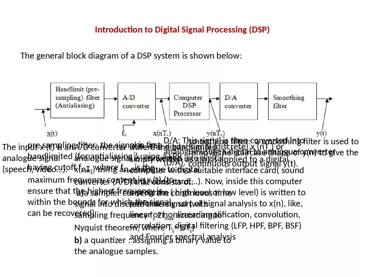
  The general block diagram of a DSP system is shown below The input x t is an analogue signal speech video pre sampling filter the signal is first bandlimited for antialiasing using a LPF having cutoff f ID: 1030799

time system signal dsp system time dsp signal bounded digital stable analogue systems causal linear values input output function

Share:

Link:

Embed:

Download Presentation from below link

Download Presentation The PPT/PDF document "Introduction to Digital Signal Processin..." is the property of its rightful owner. Permission is granted to download and print the materials on this web site for personal, non-commercial use only, and to display it on your personal computer provided you do not modify the materials and that you retain all copyright notices contained in the materials. By downloading content from our website, you accept the terms of this agreement.


Presentation Transcript

1. Introduction to Digital Signal Processing (DSP) The general block diagram of a DSP system is shown below:The input x (t) is an analogue signal (speech, video…). pre sampling filter: the signal is first bandlimited (for antialiasing*) using a LPF having cutoff fmax, where fmax is the maximum frequency content in x (t) (to ensure that the highest frequency is within the bounds for which the signal can be recovered)A/D converter :where the bandlimited analogue signal is converted into digital x(nTs) using an analogue to digital converter (A/D) that consists of: a)a sampler converts the continuous time signal into discrete time signal (with sampling frequency fs2fmax according to Nyquist theorem, where Ts=1/fs)b) a quantizer : assigning a binary value to the analogue samples. DSP: The digital signal (discrete) x (nTs) or simply written as x(n) is applied to a digital computer with a suitable interface card( sound card, video card,…). Now, inside this computer a program ( high level or low level) is written to perform any sort of signal analysis to x(n), like, linear or nonlinear amplification, convolution, correlation, digital filtering (LFP, HPF, BPF, BSF) and Fourier spectral analysisD/A: This signal is then converted into analogue using a digital to analogue converter (D/A).smoothing filter: a smoothing filter is used to remove the staircase shape of y(n) to give the continuous output signal y(t).

2. Classification of DSP systems:According to the relation between the output y(n) and the input x(n), any DSP system can be classified according to the following:1-Linearity:A DSP system is called linear if the superposition theorem applies. Superposition means that sum of the input= sum of the output.  Example1 if y(n)= 2x(n) which is a simple DSP system representing an amplifier with gain=2This DSP system is linear since superposition applies here, if x(n)=x1(n)+x2(n), then:y(n)=2[x1(n)+x2(n)]=2 x1(n)+2x2(n)=y1(n)+y2(n), where y1(n) and y2(n) are the outputs due to x1(n) and x2(n) if they are applied one at a time.

3. Example2 y(n)=3e0.2x(n) which is a DSP system representing an exponential amplifier, now if x(n)=x1(n)+x2(n), then:y(n)=3e0.2[x1(n)+x2(n)]= 3e0.2x1(n) e0.2x2(n)≠ y1(n)+y2(n), this system is nonlinearNote : examples for the nonlinear systems are: y(n)= ln(x(n)), y(n)=sin(x(n)), y(n)=1/ x(n) , y(n)= (x(n))2 2-Causality: A DSP system is said to be causal if the present value of y [ i.e. y(n)] is not a function of some future values of x [i.e. x(n+i), i, +ve integer] or some future values of y [i.e. y(n+i), i, +ve integer]. The causal DSP system that is physically realizable is that system where y(n) is a function of present value of x(n) or some previous values of x [i.e x(n-i) ,i, +ve integer] or some previous values of y [i.e. y(n-i), i +ve integer].In other words, a causal system is one where response does not begin before the input signal is appliedExample1: if y(n)=3x(n)-2x(n-1)+y(n-3)+ex(n) which is not linear due to the exponential term but it is causal since y(n) is not a function of some future terms of x or y. Example2: y(n)=x(n+1)-x(n)+3y(n+3) is not causal and is not physically realizable since y(n) depends on some future values of x and y, [these are x(n+1)) and y(n+3)].Note : examples of the noncausal systems are: y(n)=x(n+1), y(n)=x(n2) , y(n)=x(-n), y(n)=x│n│.

4. 3-Stability:A DSP system is said to be stable if the O/P is bounded for bounded I/P (bounded input gives bounded output BIBO). Ex1: if y(n)=2x(n)-0.5x(n-1)if |x(n)|<G where G is finite, then |y(n)|<2G-0.5G or |y(n)|<1.5G. hence if x(n) is bounded by G then y(n) is also bounded i.e. the system is stable. Ex2: y(n)=ex(n-1) This system is a nonlinear causal system. if |x(n)|<G, then |y(n)|<eG and if G is finite, then y(n) is bounded, i.e., the system is stable.Stability of linear DSP system can be studied usually in terms of transfer function in z-domain, H(z)=Y(z)/X(z)Where the z-transforms of x(n) and y(n) are: If H(z) has pole(s) outside the unit circle (|z|=1), then the system is unstable, otherwise, it is a stable system. Poles on the unit circle gives critically stable

5. Ex: If y(n)=2x(n-1)—3x(n). Check if this system is stable or not.Solution: Taking Z-transform of both sides, get:Y(z)=2z-1X(z)-3X(z) (using shift property of z-transform)Or Y(z)/X(z)=H(z)=2z-1-3 or: H(z)=(2-3z)/z which has a single pole at z=0(inside the unit circle), hence this system is stable.Ex: check the stability of the system: y(n)=x(n)+2y(n-1), Solution: As before, taking the z-transform of both sides and using the shift property, then :Y(z)=X(z)+2z-1Y(z), or Y(z)[1-2z-1]=X(z), then:H(z)=Y(z)/X(z)=1/(1-2z-1)=z/(z-2) which has a pole at z=2(outside the unit circle, hence this system is unstable.

6. 4-Time Variant-Time Invariant DSP system:A time variant system is that system with time varying characteristics that depends on the time index nExample1: y(n)=n x(n) is a time variant system. In fact, this system is an amplifier having variable gain with time.Example2: Classify the following DSP system for linearity, causality, stability and time invariant:y(n)=2e-x(n-1) This system is *nonlinear, *causal, *stable system*time invariant since its characteristics do not change with time index n.

7. Ex: Classify the following DSP system for linearity, causality, stability and time invariant: y(n)=2ex(n)-n x(n-2) + y(n-2).This system is:-nonlinear due to the exponential term.-casual since y(n) does not depend on some future terms of x or y-unstable due to the term n x(n-2) which is unbounded with time index n even if x is bounded-time variant due to the n x(n-2) term.Homework: classify the following DSP systems for linearity, causality, time-invariance and stability: a) y[n] = 3 x(n) – 4 x(n-1) b) y[n] = 2 y(n-1) + x(n+2) c) y[n] = n x(n) d) y[n] = cos (x(n)) e) y[n] = log10 (x(n)) f) y[n] = x[n]4

8. Input/output relations of the linear systems:a) Analogue (continuous)systemsWhere :h(t) is the impulse response and t is the time indexH(w) is the transfer function which is the Fourier transform of h(t) y(t)=x(t)  h(t)Where  is the convolutionAlso: Y(w)=X(w) H(w)

9. b) Discrete (digital) systemsh(n) is the impulse response of the System,where n is the time indexH(z) is its transfer function:H(z)=Y(z)/X(z)And:y(n)=x(n)  h(n)

10. DSP systems are classified according to their impulse responses h(n) into: FIR (Finite Impulse Response) IIR(Infinite Impulse Response)

11. Discrete convolution Methods:1- Graphical method: This includes the basic convolution steps: - reversing in time using k as time index, -shifting by n samples, -multiplication of the corresponding samples, -addition

12. And so on, shifting of h(n) (left and right) until the overlapping between x(k) and h(n-k) disappears giving 0's at the output y(n).2-Tabular Method: This is a very simple method used for FIR systems with finite number of samples x(n). A rectangular table with N1 rows (no of elements in h(n)) N2 columns(no of elements in x(n)), or visa versa, is arranged. Then, the cross multiplications are carried out. The sum of multiplications diagonally will give the values of y(n).Ex: repeat previous example using tabular method.