To illustrate Excels most popular financial functions we consider a loan with monthly payments an annual interest rate of 6 a 20year duration a present value of 150000 amount borrowed and a future value of 0 thats what you hope to achieve when you pay off a loan ID: 714325
Download Presentation The PPT/PDF document "MS EXCEL PART 4 Financial Functions" is the property of its rightful owner. Permission is granted to download and print the materials on this web site for personal, non-commercial use only, and to display it on your personal computer provided you do not modify the materials and that you retain all copyright notices contained in the materials. By downloading content from our website, you accept the terms of this agreement.
Slide1
MS EXCEL
PART 4Slide2
Financial Functions
To illustrate
Excel's
most popular financial functions, we consider a loan with monthly payments, an annual interest rate of 6%, a 20-year duration, a present value of $150,000 (amount borrowed) and a future value of 0 (that's what you hope to achieve when you pay off a loan).We make monthly payments, so we use 6%/12 = 0.5% for Rate and 20*12 = 240 for Nper (total number of periods). If we make annual payments on the same loan, we use 6% for Rate and 20 for Nper.PmtSelect cell A2 and insert the PMT function.Slide3
Note: The last two arguments are optional. For loans the
Fv
can be omitted (the future value of a loan equals 0, however, it's included here for clarification). If Type is omitted, it is assumed that payments are due at the end of the period.
Result. The monthly payment equals $1,074.65.Tip: when working with financial functions in Excel, always ask yourself the question, am I making a payment (negative) or am I receiving money (positive)? We pay off a loan of $150,000 (positive, we received that amount) and we make monthly payments of $1,074.65 (negative, we pay).Slide4
Rate
If Rate is the only unknown variable, we can use the RATE function to calculate the interest rate.
Rate
NperOr the NPER function. If we make monthly payments of $1,074.65 on a 20-year loan, with an annual interest rate of 6%, it takes 240 months to pay off this loan.
We
already knew this, but we can change the monthly payment now to see how this affects the total number of periods.Slide5
nper
Conclusion: if we make monthly payments of $2,074.65, it takes less than 90 months to pay off this loan.
Pv
Or the PV (Present Value) function. If we make monthly payments of $1,074.65 on a 20-year loan, with an annual interest rate of 6%, how much can we borrow? You already know the answer.Slide6
Fv
If
we make monthly payments of $1,074.65 on a 20-year loan, with an annual interest rate of 6%, do we pay off this loan? Yes.
But, if we make monthly payments of only $1,000.00, we still have debt after 20 years.Slide7
Charts
A simple
chart
in Excel can say more than a sheet full of numbers. As you'll see, creating charts is very easy.Create a ChartTo create a line chart, execute the following steps.1. Select the range A1:D7.2. On the Insert tab, in the Charts group, choose Line, and select Line with Markers.Slide8
Result:Slide9
Change Chart Type
You can easily change to a different type of chart at any time.
1. Select the chart.
2. On the Insert tab, in the Charts group, choose Column, and select Clustered Column.Slide10
Result:Slide11
Switch Row/Column
If
you want the animals, displayed on the vertical axis, to be displayed on the horizontal axis instead, execute the following steps.
1. Select the chart. The Chart Tools contextual tab activates.2. On the Design tab, click Switch Row/Column.Result:Slide12
Chart Title
To add a chart title, execute the following steps.
1. Select the chart. The Chart Tools contextual tab activates.
2. On the Layout tab, click Chart Title, Above Chart.Slide13
3. Enter a title. For example, Population.
Result:Slide14
Legend Position
By
default, the legend appears to the right of the chart. To move the legend to the bottom of the chart, execute the following steps.
1. Select the chart. The Chart Tools contextual tab activates.2. On the Layout tab, click Legend, Show Legend at Bottom.Slide15
Result:
You can use data labels to focus your readers' attention on a single data series or data point.
1. Select the chart. The Chart Tools contextual tab activates.
2. Click an orange bar to select the Jun data series. Click again on an orange bar to select a single data point.3. On the Layout tab, click Data Labels, Outside End.Slide16
Data LabelsSlide17
Result:Slide18
Pivot Table
Pivot tables
are one of
Excel's most powerful features. A pivot table allows you to extract the significance from a large, detailed data set.Our data set consists of 214 rows and 6 fields. Order ID, Product, Category, Amount, Date and Country.Slide19
Insert a Pivot Table
To insert a
pivot table
, execute the following steps.1. Click any single cell inside the data set.2. On the Insert tab, click PivotTable.The following dialog box appears. Excel automatically selects the data for you. The default location for a new pivot table is New Worksheet.
3. Click OK.Slide20
Drag fields
The
PivotTable field list
appears.To get the total amount exported of each product, drag the following fields to the different areas.1. Product Field to the Row Labels area.2. Amount Field to the Values area.3. Country Field to the Report Filter area.Slide21
Below you can find the pivot table. Bananas are our main export product. That's how easy pivot tables can be!Slide22
Sort
To get Banana at the top of the list, sort the pivot table.
1
. Click any cell inside the Total column.2. The PivotTable Tools contextual tab activates. On the Options tab, click the Sort Largest to Smallest button (ZA).Slide23
Result.Slide24
Filter
Because
we added the Country field to the Report Filter area, we can filter this pivot table by Country. For example, which products do we export the most to France?
1. Click the filter drop-down and select France.Result. Apples are our main export product to France.Note: you can use the standard filter (triangle next to Product) to only show the totals of specific products.Slide25
Change Summary Calculation
By
default, Excel summarizes your data by either summing or counting the items. To change the type of calculation that you want to use, execute the following steps.
1. Click any cell inside the Total column.2. Right click and click on Value Field Settings...Slide26
3. Choose the type of calculation you want to use. For example, click Count.Slide27
4. Click OK.
Result. 16 out of the 28 orders to France were 'Apple' orders.Slide28
Two-dimensional Pivot Table
If you drag a field to the Row Labels area and Column Labels area, you can create a two-dimensional pivot table. For example, to get the total amount exported to each country, of each product, drag the following fields to the different areas.
1. Country Field to the Row Labels area.
2. Product Field to the Column Labels area.3. Amount Field to the Values area.4. Category Field to the Report Filter area.Slide29
Below you can find the two-dimensional pivot table.Slide30
To easily compare these numbers, create a
pivot chart
and apply a filter. Maybe this is one step too far for you at this stage, but it shows you one of the many other powerful pivot table features Excel has to offer.