1 Derivatives Advanced Topics: Interest Rate

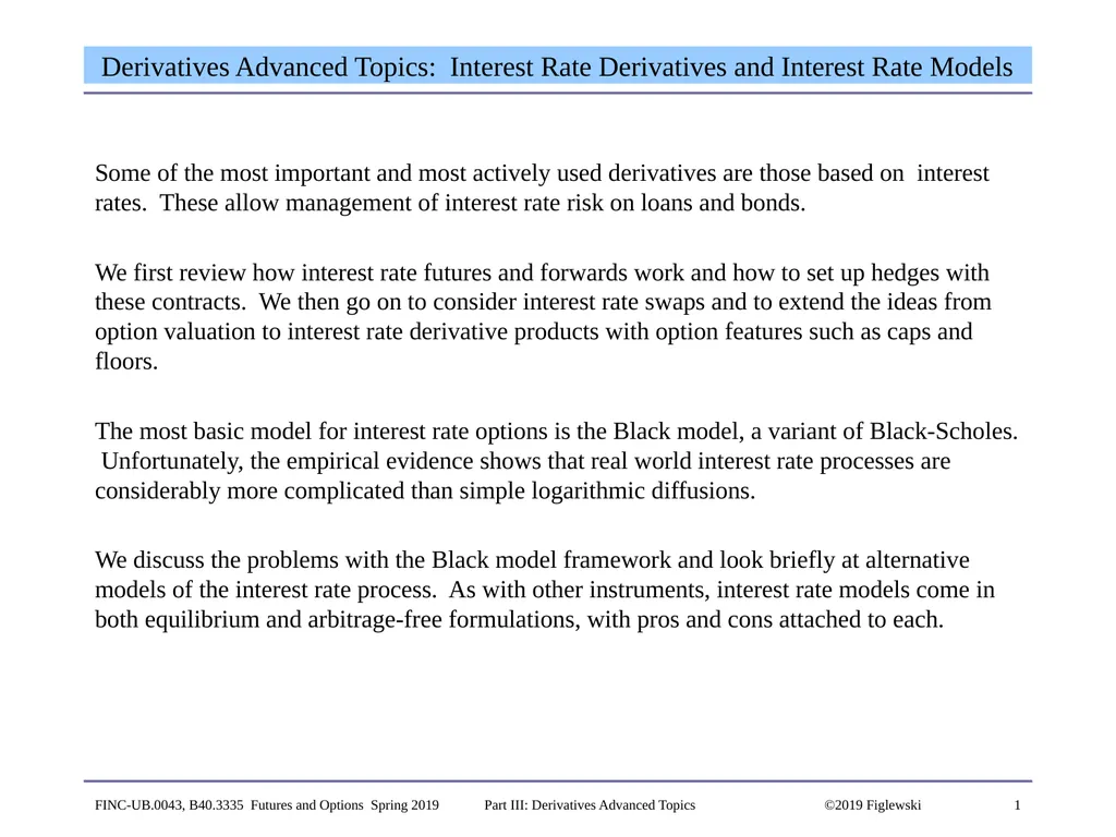
slide1. 1 Derivatives Advanced Topics: Interest Rate Derivatives and Interest Rate Models Some of the most important and most actively used derivatives are those based on interest rates. These allow management of interest rate risk on loans and bonds.

We first review how interest rate futures and forwards work and how to set up hedges with these contracts. We then go on to consider interest rate swaps and to extend the ideas from option valuation to interest rate derivative products with option features such as caps and floors.

The most basic model for interest rate options is the Black model, a variant of Black-Scholes. Unfortunately, the empirical evidence shows that real world interest rate processes are considerably more complicated than simple logarithmic diffusions.

We discuss the problems with the Black model framework and look briefly at alternative models of the interest rate process. As with other instruments, interest rate models come in both equilibrium and arbitrage-free formulations, with pros and cons attached to each. FINC-UB.0043, B40.3335 Futures and Options Spring 2019 Part III: Derivatives Advanced Topics ©2019 Figlewski<br>
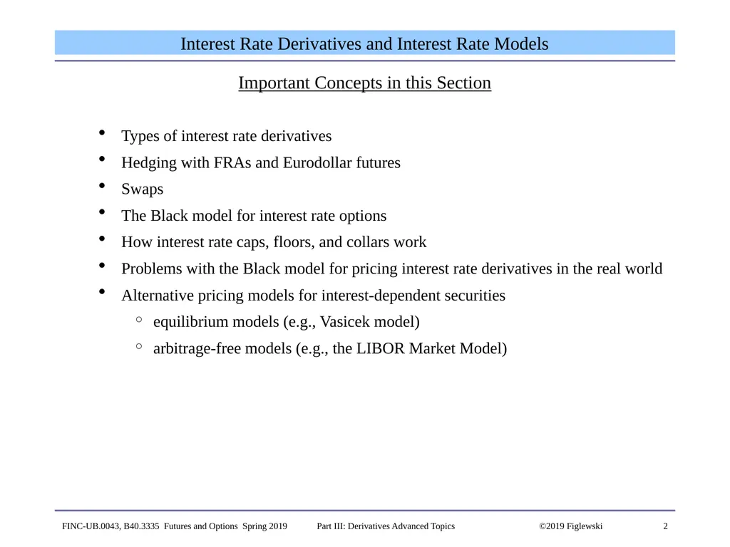
slide2. 2 Interest Rate Derivatives and Interest Rate Models Important Concepts in this Section

Types of interest rate derivatives
Hedging with FRAs and Eurodollar futures
Swaps
The Black model for interest rate options
How interest rate caps, floors, and collars work
Problems with the Black model for pricing interest rate derivatives in the real world
Alternative pricing models for interest-dependent securities
equilibrium models (e.g., Vasicek model)
arbitrage-free models (e.g., the LIBOR Market Model) FINC-UB.0043, B40.3335 Futures and Options Spring 2019 Part III: Derivatives Advanced Topics ©2019 Figlewski<br>
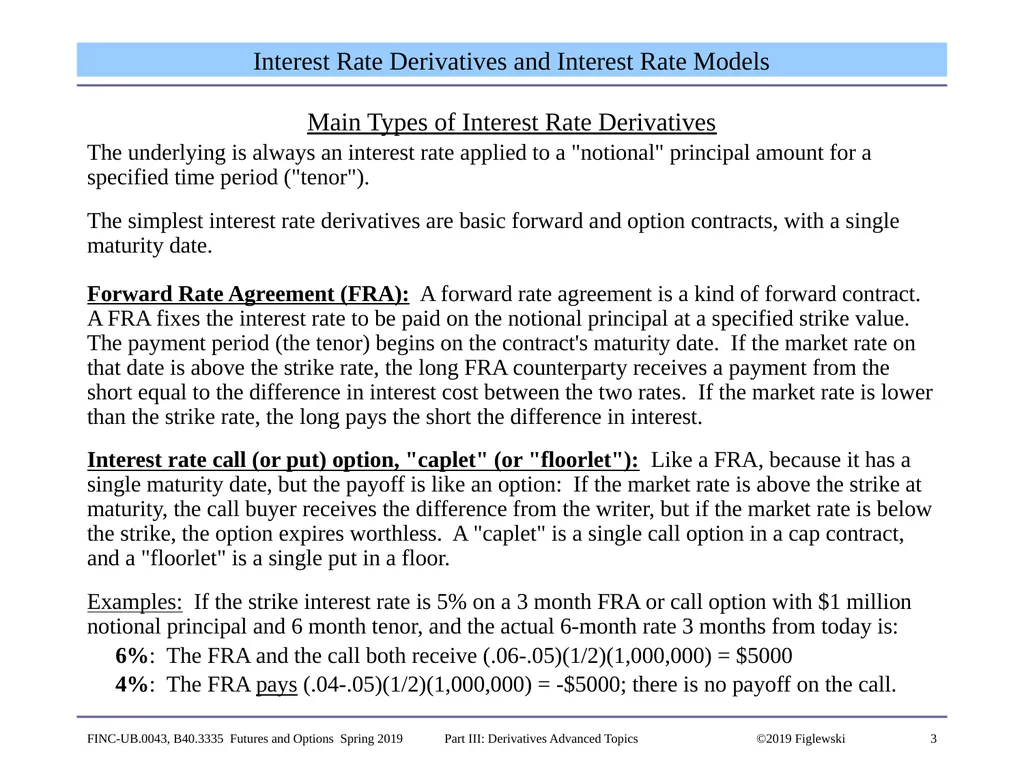
slide3. 3 Interest Rate Derivatives and Interest Rate Models Main Types of Interest Rate Derivatives
The underlying is always an interest rate applied to a "notional" principal amount for a specified time period ("tenor").

The simplest interest rate derivatives are basic forward and option contracts, with a single maturity date.

Forward Rate Agreement (FRA): A forward rate agreement is a kind of forward contract. A FRA fixes the interest rate to be paid on the notional principal at a specified strike value. The payment period (the tenor) begins on the contract's maturity date. If the market rate on that date is above the strike rate, the long FRA counterparty receives a payment from the short equal to the difference in interest cost between the two rates. If the market rate is lower than the strike rate, the long pays the short the difference in interest.

Interest rate call (or put) option, "caplet" (or "floorlet"): Like a FRA, because it has a single maturity date, but the payoff is like an option: If the market rate is above the strike at maturity, the call buyer receives the difference from the writer, but if the market rate is below the strike, the option expires worthless. A "caplet" is a single call option in a cap contract, and a "floorlet" is a single put in a floor.

Examples: If the strike interest rate is 5% on a 3 month FRA or call option with $1 million notional principal and 6 month tenor, and the actual 6-month rate 3 months from today is:
6%: The FRA and the call both receive (.06-.05)(1/2)(1,000,000) = $5000
4%: The FRA pays (.04-.05)(1/2)(1,000,000) = -$5000; there is no payoff on the call. FINC-UB.0043, B40.3335 Futures and Options Spring 2019 Part III: Derivatives Advanced Topics ©2019 Figlewski<br>
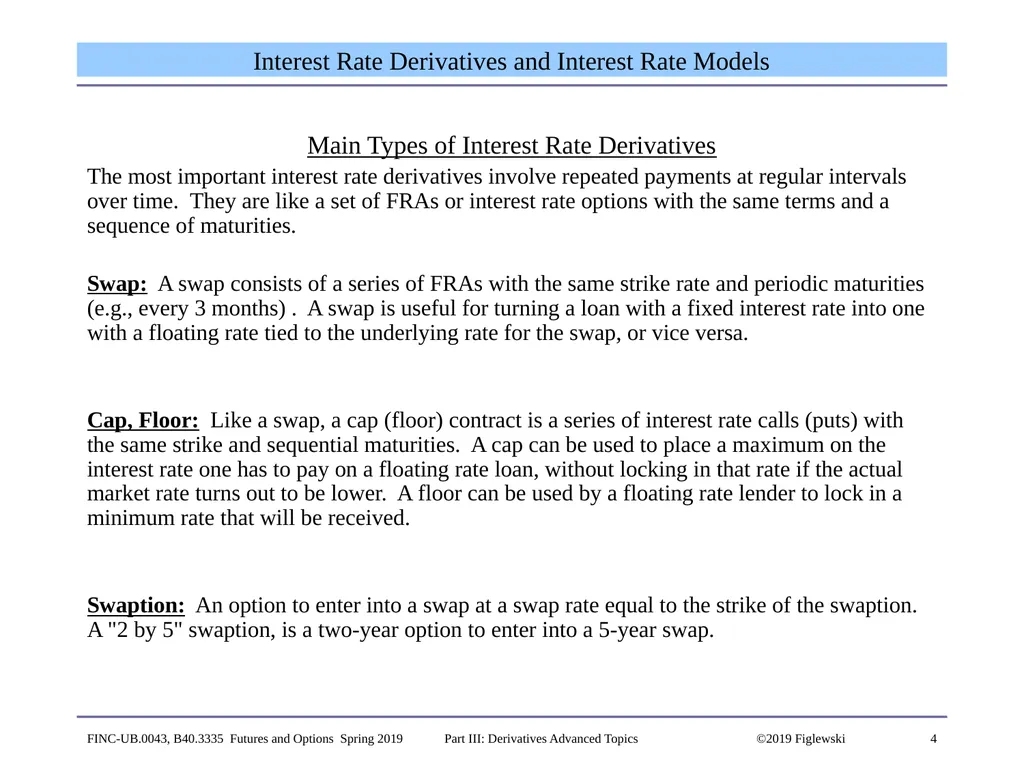
slide4. 4 Interest Rate Derivatives and Interest Rate Models Main Types of Interest Rate Derivatives
The most important interest rate derivatives involve repeated payments at regular intervals over time. They are like a set of FRAs or interest rate options with the same terms and a sequence of maturities.

Swap: A swap consists of a series of FRAs with the same strike rate and periodic maturities (e.g., every 3 months) . A swap is useful for turning a loan with a fixed interest rate into one with a floating rate tied to the underlying rate for the swap, or vice versa.

Cap, Floor: Like a swap, a cap (floor) contract is a series of interest rate calls (puts) with the same strike and sequential maturities. A cap can be used to place a maximum on the interest rate one has to pay on a floating rate loan, without locking in that rate if the actual market rate turns out to be lower. A floor can be used by a floating rate lender to lock in a minimum rate that will be received.

Swaption: An option to enter into a swap at a swap rate equal to the strike of the swaption. A "2 by 5" swaption, is a two-year option to enter into a 5-year swap. FINC-UB.0043, B40.3335 Futures and Options Spring 2019 Part III: Derivatives Advanced Topics ©2019 Figlewski<br>
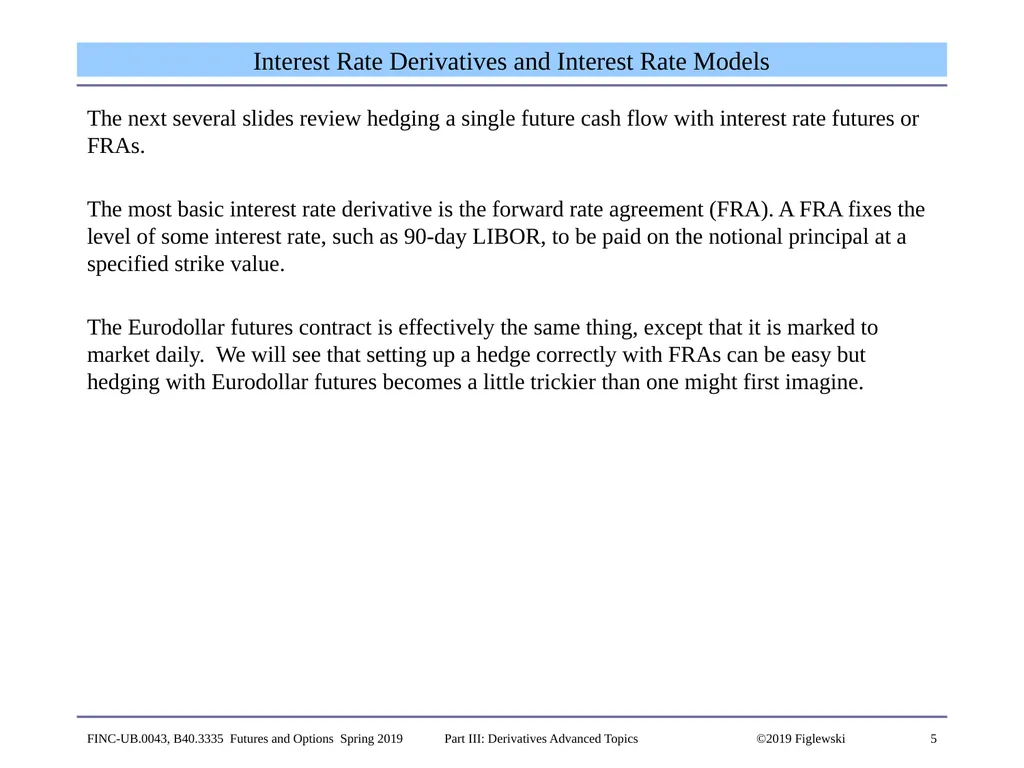
slide5. 5 Interest Rate Derivatives and Interest Rate Models The next several slides review hedging a single future cash flow with interest rate futures or FRAs.

The most basic interest rate derivative is the forward rate agreement (FRA). A FRA fixes the level of some interest rate, such as 90-day LIBOR, to be paid on the notional principal at a specified strike value.

The Eurodollar futures contract is effectively the same thing, except that it is marked to market daily. We will see that setting up a hedge correctly with FRAs can be easy but hedging with Eurodollar futures becomes a little trickier than one might first imagine. FINC-UB.0043, B40.3335 Futures and Options Spring 2019 Part III: Derivatives Advanced Topics ©2019 Figlewski<br>
slide6. 6 Interest Rate Derivatives and Interest Rate Models Recall that:

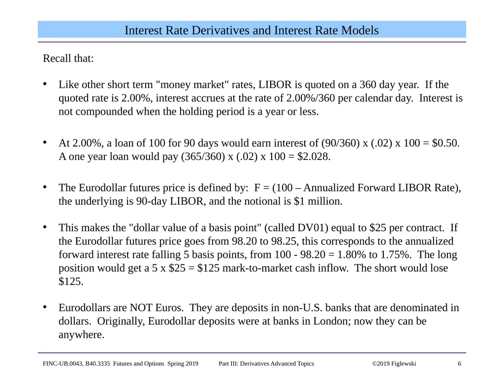
Like other short term "money market" rates, LIBOR is quoted on a 360 day year. If the quoted rate is 2.00%, interest accrues at the rate of 2.00%/360 per calendar day. Interest is not compounded when the holding period is a year or less.

At 2.00%, a loan of 100 for 90 days would earn interest of (90/360) x (.02) x 100 = $0.50. A one year loan would pay (365/360) x (.02) x 100 = $2.028.

The Eurodollar futures price is defined by: F = (100 – Annualized Forward LIBOR Rate), the underlying is 90-day LIBOR, and the notional is $1 million.

This makes the "dollar value of a basis point" (called DV01) equal to $25 per contract. If the Eurodollar futures price goes from 98.20 to 98.25, this corresponds to the annualized forward interest rate falling 5 basis points, from 100 - 98.20 = 1.80% to 1.75%. The long position would get a 5 x $25 = $125 mark-to-market cash inflow. The short would lose $125.

Eurodollars are NOT Euros. They are deposits in non-U.S. banks that are denominated in dollars. Originally, Eurodollar deposits were at banks in London; now they can be anywhere. FINC-UB.0043, B40.3335 Futures and Options Spring 2019 Part III: Derivatives Advanced Topics ©2019 Figlewski<br>
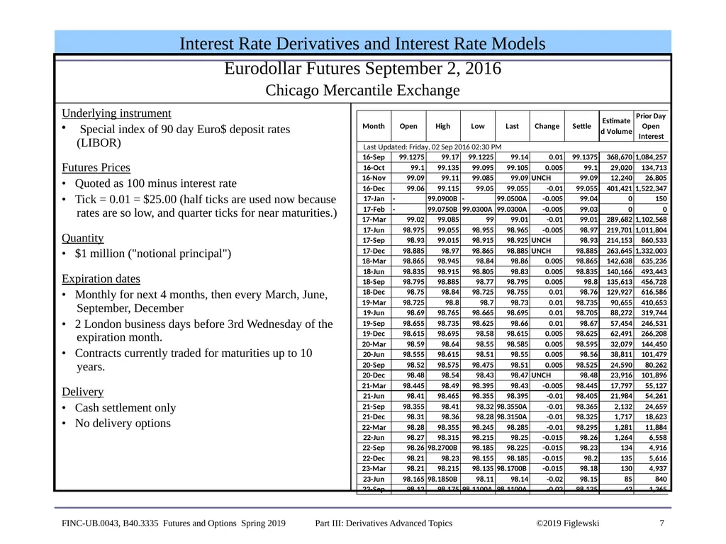
slide7. FINC-UB.0043, B40.3335 Futures and Options Spring 2019 Part III: Derivatives Advanced Topics ©2019 Figlewski 7 Interest Rate Derivatives and Interest Rate Models<br>
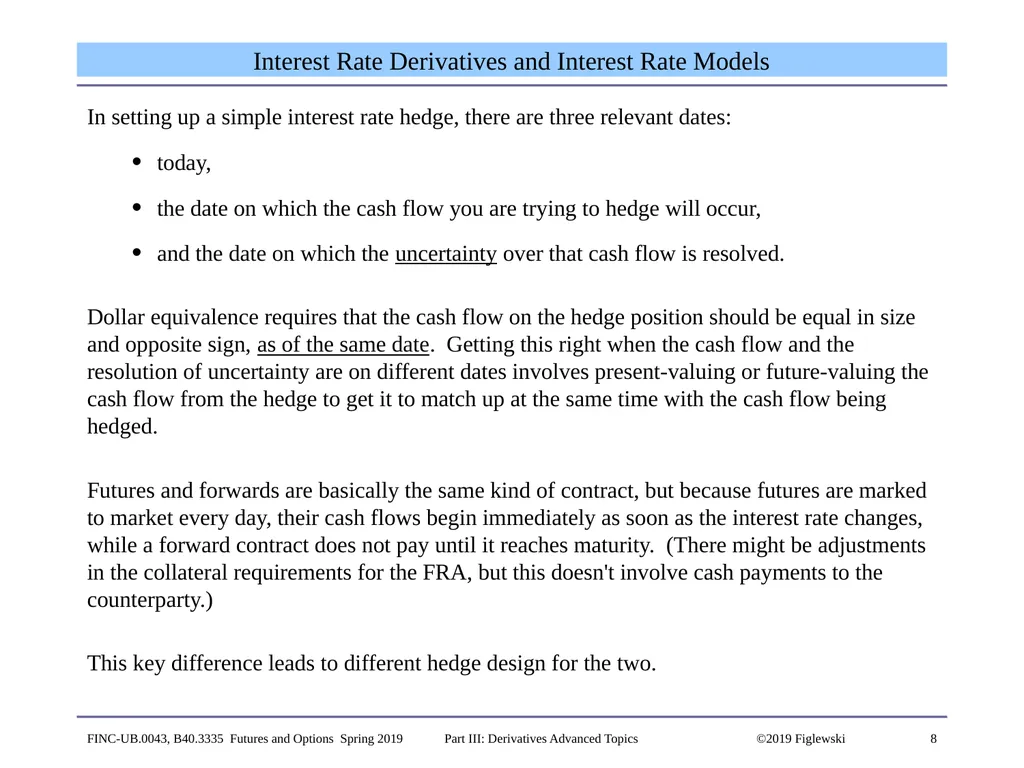
slide8. 8 Interest Rate Derivatives and Interest Rate Models In setting up a simple interest rate hedge, there are three relevant dates:
today,
the date on which the cash flow you are trying to hedge will occur,
and the date on which the uncertainty over that cash flow is resolved.

Dollar equivalence requires that the cash flow on the hedge position should be equal in size and opposite sign, as of the same date. Getting this right when the cash flow and the resolution of uncertainty are on different dates involves present-valuing or future-valuing the cash flow from the hedge to get it to match up at the same time with the cash flow being hedged.

Futures and forwards are basically the same kind of contract, but because futures are marked to market every day, their cash flows begin immediately as soon as the interest rate changes, while a forward contract does not pay until it reaches maturity. (There might be adjustments in the collateral requirements for the FRA, but this doesn't involve cash payments to the counterparty.)

This key difference leads to different hedge design for the two. FINC-UB.0043, B40.3335 Futures and Options Spring 2019 Part III: Derivatives Advanced Topics ©2019 Figlewski<br>
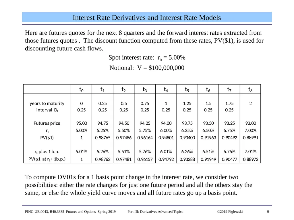
slide9. 9 Interest Rate Derivatives and Interest Rate Models Here are futures quotes for the next 8 quarters and the forward interest rates extracted from those futures quotes . The discount function computed from these rates, PV($1), is used for discounting future cash flows.
Spot interest rate: r0 = 5.00%
Notional: V = $100,000,000

To compute DV01s for a 1 basis point change in the interest rate, we consider two possibilities: either the rate changes for just one future period and all the others stay the same, or else the whole yield curve moves and all future rates go up a basis point. FINC-UB.0043, B40.3335 Futures and Options Spring 2019 Part III: Derivatives Advanced Topics ©2019 Figlewski<br>
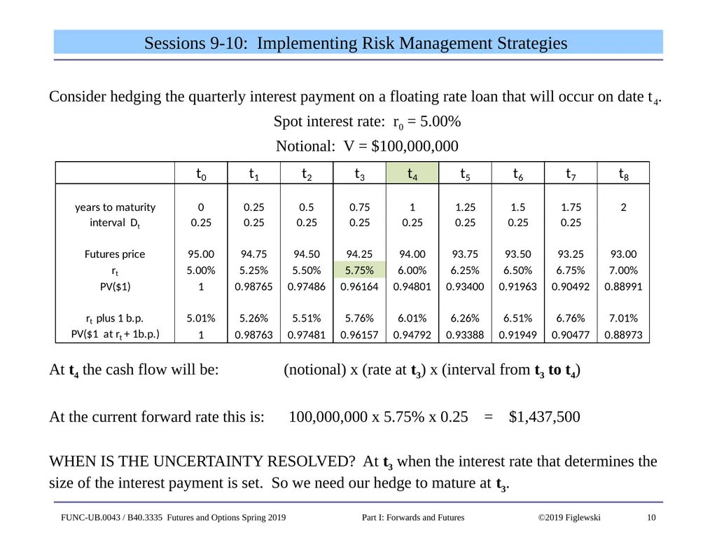
slide10. 10 Sessions 9-10: Implementing Risk Management Strategies Consider hedging the quarterly interest payment on a floating rate loan that will occur on date t4.
Spot interest rate: r0 = 5.00%
Notional: V = $100,000,000

At t4 the cash flow will be: (notional) x (rate at t3) x (interval from t3 to t4)

At the current forward rate this is: 100,000,000 x 5.75% x 0.25 = $1,437,500

WHEN IS THE UNCERTAINTY RESOLVED? At t3 when the interest rate that determines the size of the interest payment is set. So we need our hedge to mature at t3. FUNC-UB.0043 / B40.3335 Futures and Options Spring 2019 Part I: Forwards and Futures ©2019 Figlewski<br>
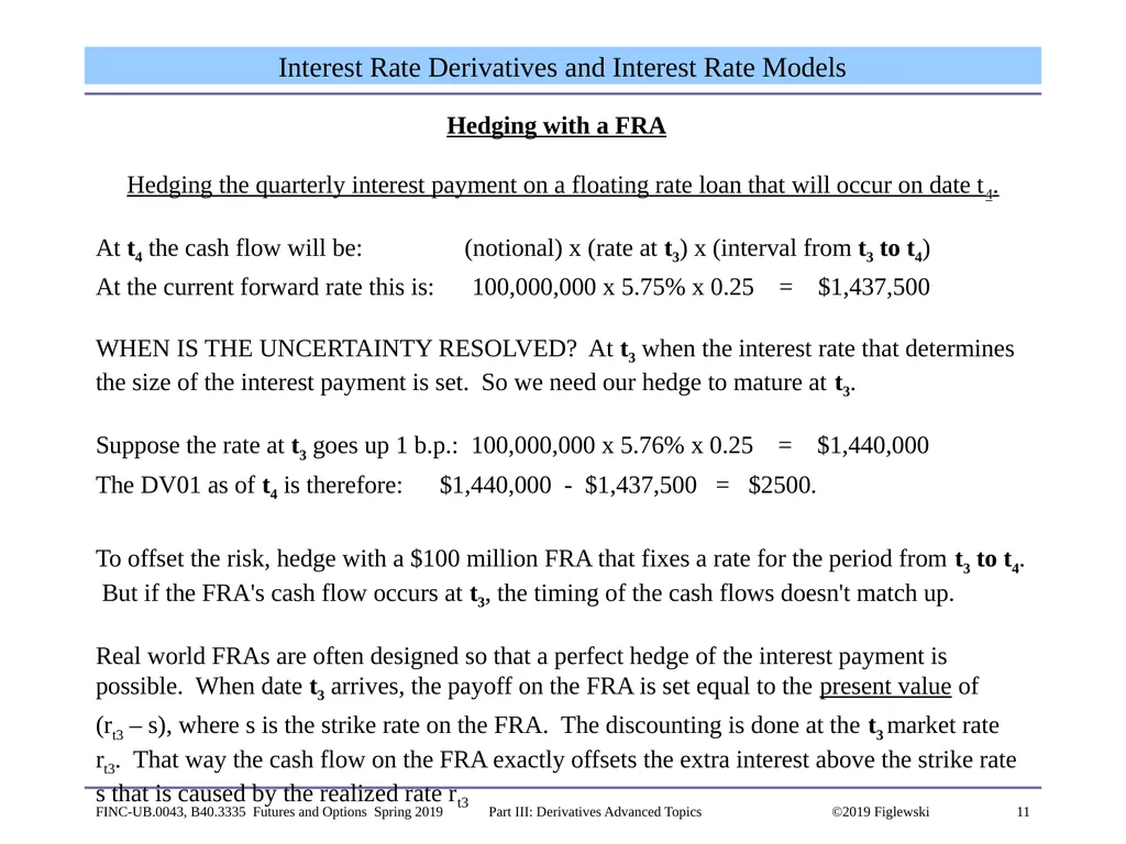
slide11. 11 Interest Rate Derivatives and Interest Rate Models Hedging with a FRA

Hedging the quarterly interest payment on a floating rate loan that will occur on date t4.

At t4 the cash flow will be: (notional) x (rate at t3) x (interval from t3 to t4)
At the current forward rate this is: 100,000,000 x 5.75% x 0.25 = $1,437,500

WHEN IS THE UNCERTAINTY RESOLVED? At t3 when the interest rate that determines the size of the interest payment is set. So we need our hedge to mature at t3.

Suppose the rate at t3 goes up 1 b.p.: 100,000,000 x 5.76% x 0.25 = $1,440,000
The DV01 as of t4 is therefore: $1,440,000 - $1,437,500 = $2500.

To offset the risk, hedge with a $100 million FRA that fixes a rate for the period from t3 to t4. But if the FRA's cash flow occurs at t3, the timing of the cash flows doesn't match up.

Real world FRAs are often designed so that a perfect hedge of the interest payment is possible. When date t3 arrives, the payoff on the FRA is set equal to the present value of
(rt3 – s), where s is the strike rate on the FRA. The discounting is done at the t3 market rate rt3. That way the cash flow on the FRA exactly offsets the extra interest above the strike rate s that is caused by the realized rate rt3 FINC-UB.0043, B40.3335 Futures and Options Spring 2019 Part III: Derivatives Advanced Topics ©2019 Figlewski<br>
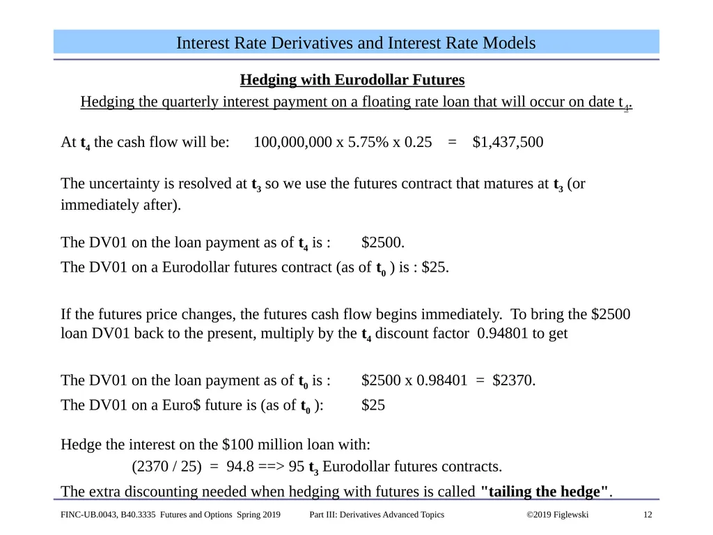
slide12. 12 Interest Rate Derivatives and Interest Rate Models Hedging with Eurodollar Futures
Hedging the quarterly interest payment on a floating rate loan that will occur on date t4.

At t4 the cash flow will be: 100,000,000 x 5.75% x 0.25 = $1,437,500

The uncertainty is resolved at t3 so we use the futures contract that matures at t3 (or immediately after).

The DV01 on the loan payment as of t4 is : $2500.
The DV01 on a Eurodollar futures contract (as of t0 ) is : $25.

If the futures price changes, the futures cash flow begins immediately. To bring the $2500 loan DV01 back to the present, multiply by the t4 discount factor 0.94801 to get

The DV01 on the loan payment as of t0 is : $2500 x 0.98401 = $2370.
The DV01 on a Euro$ future is (as of t0 ): $25

Hedge the interest on the $100 million loan with:
(2370 / 25) = 94.8 ==> 95 t3 Eurodollar futures contracts.
The extra discounting needed when hedging with futures is called "tailing the hedge". FINC-UB.0043, B40.3335 Futures and Options Spring 2019 Part III: Derivatives Advanced Topics ©2019 Figlewski<br>
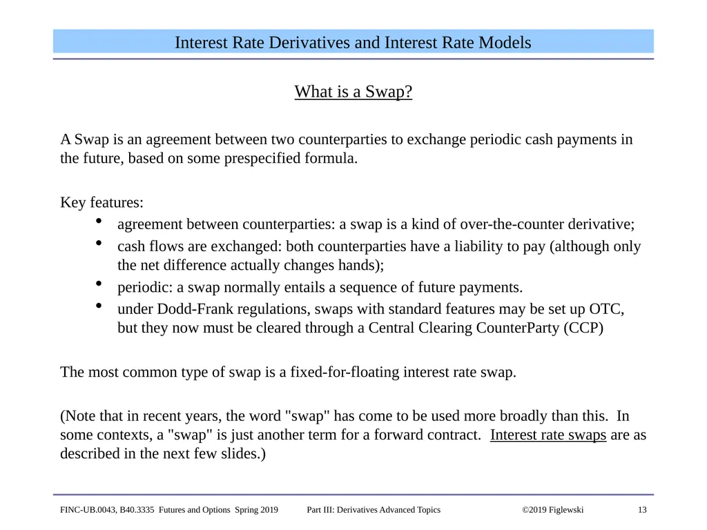
slide13. 13 Interest Rate Derivatives and Interest Rate Models What is a Swap?

A Swap is an agreement between two counterparties to exchange periodic cash payments in the future, based on some prespecified formula.

Key features:
agreement between counterparties: a swap is a kind of over-the-counter derivative;
cash flows are exchanged: both counterparties have a liability to pay (although only the net difference actually changes hands);
periodic: a swap normally entails a sequence of future payments.
under Dodd-Frank regulations, swaps with standard features may be set up OTC, but they now must be cleared through a Central Clearing CounterParty (CCP)

The most common type of swap is a fixed-for-floating interest rate swap.

(Note that in recent years, the word "swap" has come to be used more broadly than this. In some contexts, a "swap" is just another term for a forward contract. Interest rate swaps are as described in the next few slides.) FINC-UB.0043, B40.3335 Futures and Options Spring 2019 Part III: Derivatives Advanced Topics ©2019 Figlewski<br>
slide14. 14 Interest Rate Derivatives and Interest Rate Models Example of a Swap

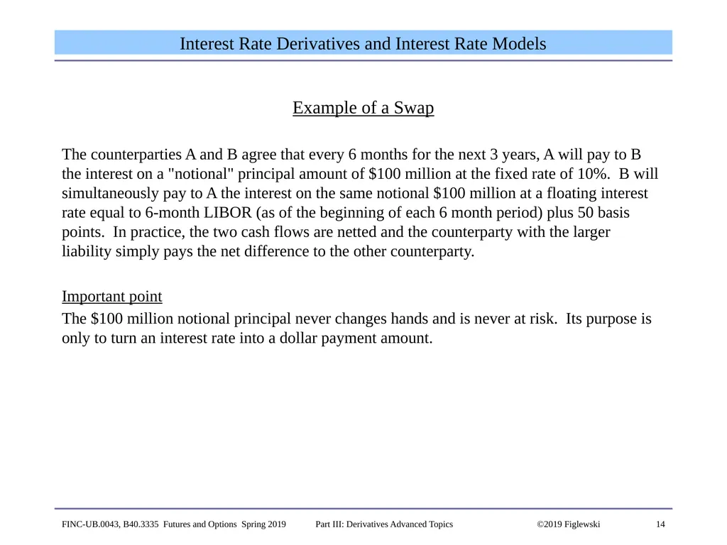
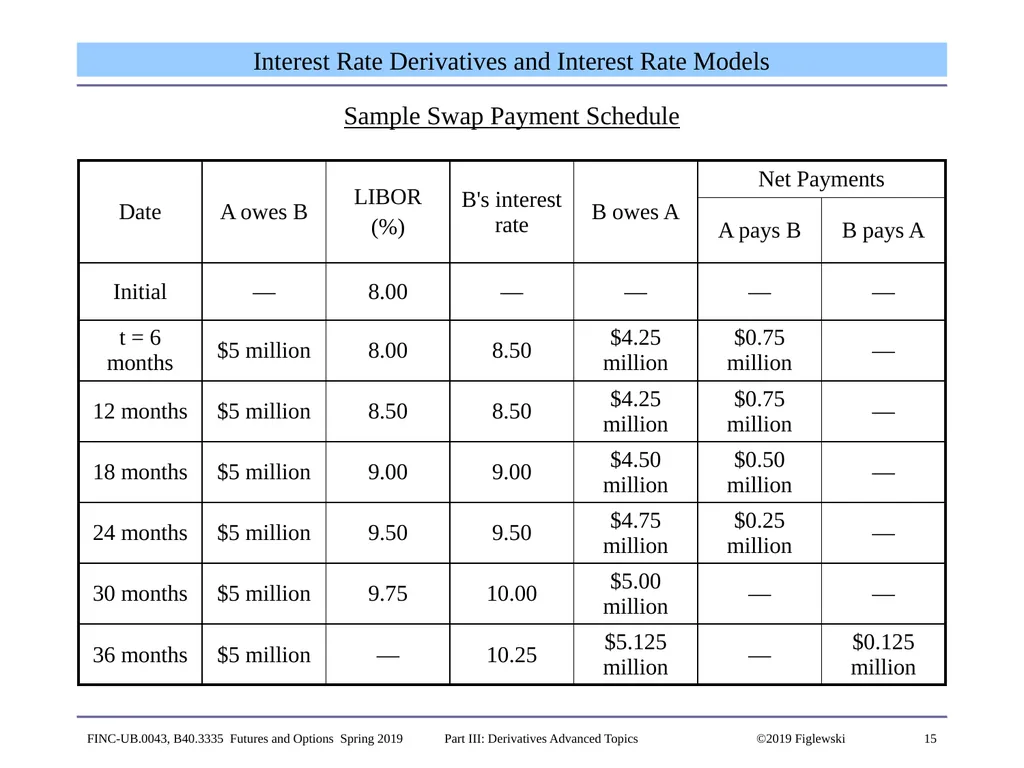
The counterparties A and B agree that every 6 months for the next 3 years, A will pay to B the interest on a "notional" principal amount of $100 million at the fixed rate of 10%. B will simultaneously pay to A the interest on the same notional $100 million at a floating interest rate equal to 6-month LIBOR (as of the beginning of each 6 month period) plus 50 basis points. In practice, the two cash flows are netted and the counterparty with the larger liability simply pays the net difference to the other counterparty.

Important point
The $100 million notional principal never changes hands and is never at risk. Its purpose is only to turn an interest rate into a dollar payment amount. FINC-UB.0043, B40.3335 Futures and Options Spring 2019 Part III: Derivatives Advanced Topics ©2019 Figlewski<br>
slide15. 15 Interest Rate Derivatives and Interest Rate Models Sample Swap Payment Schedule FINC-UB.0043, B40.3335 Futures and Options Spring 2019 Part III: Derivatives Advanced Topics ©2019 Figlewski<br>
slide16. 16 Interest Rate Derivatives and Interest Rate Models Why Swap?
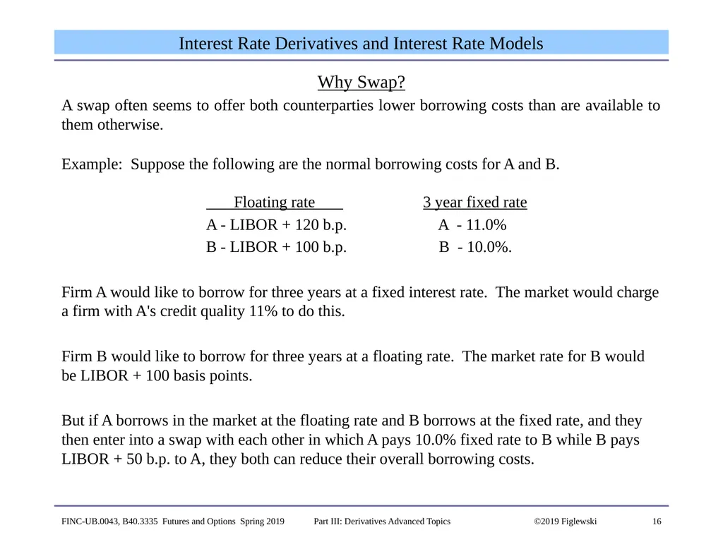
A swap often seems to offer both counterparties lower borrowing costs than are available to them otherwise.

Example: Suppose the following are the normal borrowing costs for A and B.

Floating rate 3 year fixed rate
A - LIBOR + 120 b.p. A - 11.0%
B - LIBOR + 100 b.p. B - 10.0%.

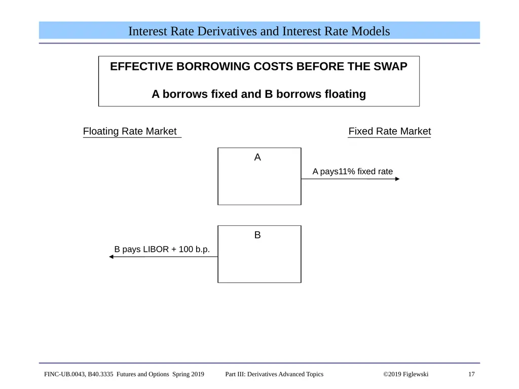
Firm A would like to borrow for three years at a fixed interest rate. The market would charge a firm with A's credit quality 11% to do this.

Firm B would like to borrow for three years at a floating rate. The market rate for B would be LIBOR + 100 basis points.

But if A borrows in the market at the floating rate and B borrows at the fixed rate, and they then enter into a swap with each other in which A pays 10.0% fixed rate to B while B pays LIBOR + 50 b.p. to A, they both can reduce their overall borrowing costs. FINC-UB.0043, B40.3335 Futures and Options Spring 2019 Part III: Derivatives Advanced Topics ©2019 Figlewski<br>
slide17. 17 Interest Rate Derivatives and Interest Rate Models B A Floating Rate Market Fixed Rate Market B pays LIBOR + 100 b.p. A pays11% fixed rate EFFECTIVE BORROWING COSTS BEFORE THE SWAP

A borrows fixed and B borrows floating FINC-UB.0043, B40.3335 Futures and Options Spring 2019 Part III: Derivatives Advanced Topics ©2019 Figlewski<br>
slide18. 18 Interest Rate Derivatives and Interest Rate Models How does this work?

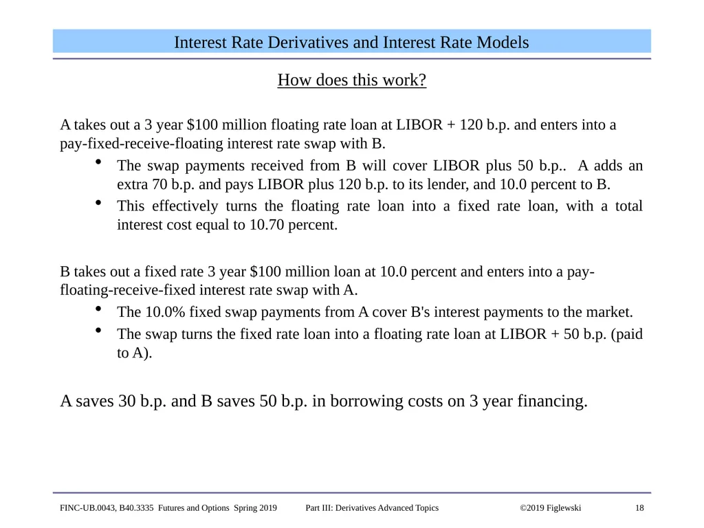
A takes out a 3 year $100 million floating rate loan at LIBOR + 120 b.p. and enters into a pay-fixed-receive-floating interest rate swap with B.
The swap payments received from B will cover LIBOR plus 50 b.p.. A adds an extra 70 b.p. and pays LIBOR plus 120 b.p. to its lender, and 10.0 percent to B.
This effectively turns the floating rate loan into a fixed rate loan, with a total interest cost equal to 10.70 percent.

B takes out a fixed rate 3 year $100 million loan at 10.0 percent and enters into a pay-floating-receive-fixed interest rate swap with A.
The 10.0% fixed swap payments from A cover B's interest payments to the market.
The swap turns the fixed rate loan into a floating rate loan at LIBOR + 50 b.p. (paid to A).

A saves 30 b.p. and B saves 50 b.p. in borrowing costs on 3 year financing. FINC-UB.0043, B40.3335 Futures and Options Spring 2019 Part III: Derivatives Advanced Topics ©2019 Figlewski<br>
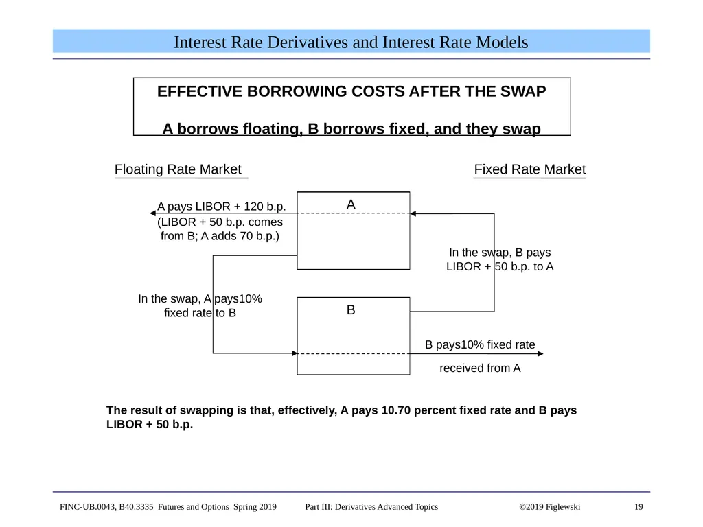
slide19. 19 Interest Rate Derivatives and Interest Rate Models B A Floating Rate Market Fixed Rate Market A pays LIBOR + 120 b.p. EFFECTIVE BORROWING COSTS AFTER THE SWAP

A borrows floating, B borrows fixed, and they swap The result of swapping is that, effectively, A pays 10.70 percent fixed rate and B pays LIBOR + 50 b.p. B pays10% fixed rate FINC-UB.0043, B40.3335 Futures and Options Spring 2019 Part III: Derivatives Advanced Topics ©2019 Figlewski<br>
slide20. 20 Interest Rate Derivatives and Interest Rate Models Are Swaps a Free Lunch?

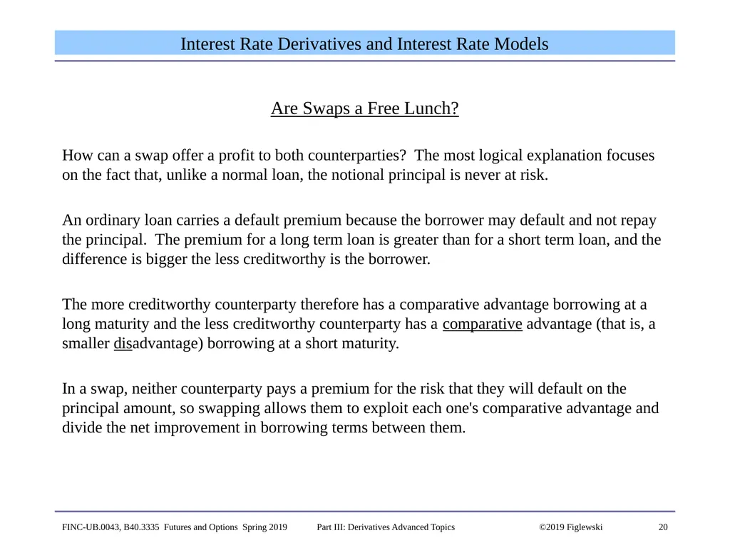
How can a swap offer a profit to both counterparties? The most logical explanation focuses on the fact that, unlike a normal loan, the notional principal is never at risk.

An ordinary loan carries a default premium because the borrower may default and not repay the principal. The premium for a long term loan is greater than for a short term loan, and the difference is bigger the less creditworthy is the borrower.

The more creditworthy counterparty therefore has a comparative advantage borrowing at a long maturity and the less creditworthy counterparty has a comparative advantage (that is, a smaller disadvantage) borrowing at a short maturity.

In a swap, neither counterparty pays a premium for the risk that they will default on the principal amount, so swapping allows them to exploit each one's comparative advantage and divide the net improvement in borrowing terms between them. FINC-UB.0043, B40.3335 Futures and Options Spring 2019 Part III: Derivatives Advanced Topics ©2019 Figlewski<br>
slide21. 21 Interest Rate Derivatives and Interest Rate Models Pricing a Swap
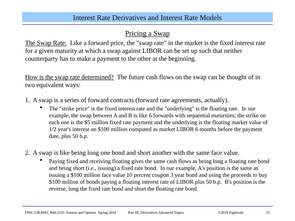
The Swap Rate: Like a forward price, the "swap rate" in the market is the fixed interest rate for a given maturity at which a swap against LIBOR can be set up such that neither counterparty has to make a payment to the other at the beginning.

How is the swap rate determined? The future cash flows on the swap can be thought of in two equivalent ways:

1. A swap is a series of forward contracts (forward rate agreements, actually).
The "strike price" is the fixed interest rate and the "underlying" is the floating rate. In our example, the swap between A and B is like 6 forwards with sequential maturities; the strike on each one is the $5 million fixed rate payment and the underlying is the floating market value of 1/2 year's interest on $100 million computed as market LIBOR 6 months before the payment date, plus 50 b.p.

2. A swap is like being long one bond and short another with the same face value.
Paying fixed and receiving floating gives the same cash flows as being long a floating rate bond and being short (i.e., issuing) a fixed rate bond. In our example, A's position is the same as issuing a $100 million face value 10 percent coupon 3 year bond and using the proceeds to buy $100 million of bonds paying a floating interest rate of LIBOR plus 50 b.p. B's position is the reverse, long the fixed rate bond and short the floating rate bond. FINC-UB.0043, B40.3335 Futures and Options Spring 2019 Part III: Derivatives Advanced Topics ©2019 Figlewski<br>
slide22. 22 Interest Rate Derivatives and Interest Rate Models Pricing a Swap
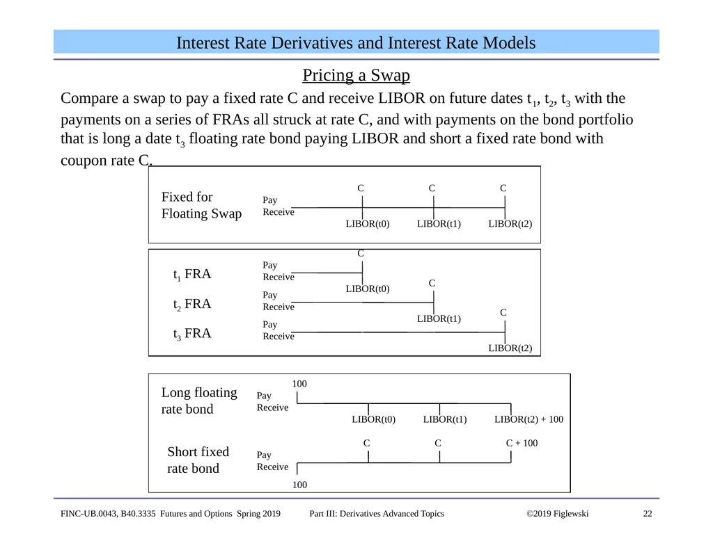
Compare a swap to pay a fixed rate C and receive LIBOR on future dates t1, t2, t3 with the payments on a series of FRAs all struck at rate C, and with payments on the bond portfolio that is long a date t3 floating rate bond paying LIBOR and short a fixed rate bond with coupon rate C. FINC-UB.0043, B40.3335 Futures and Options Spring 2019 Part III: Derivatives Advanced Topics ©2019 Figlewski<br>
slide23. 23 Interest Rate Derivatives and Interest Rate Models Pricing a Swap, p.2

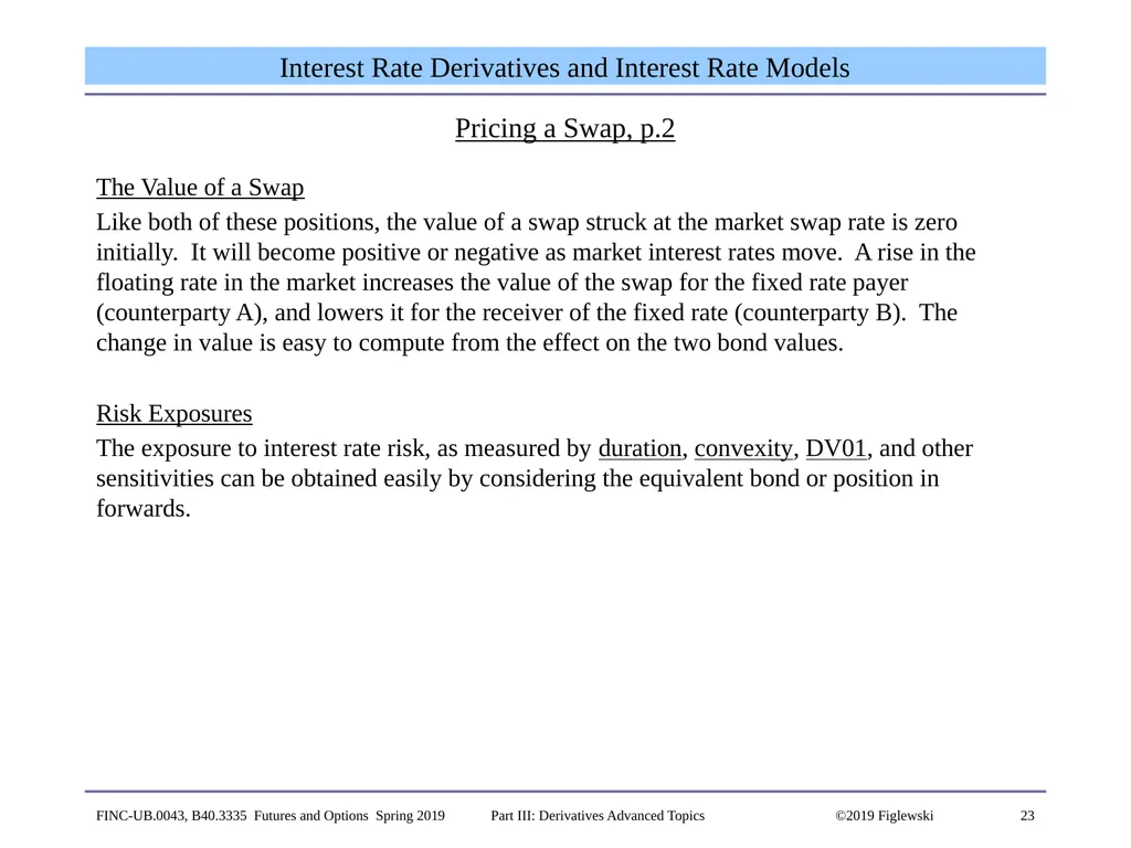
The Value of a Swap
Like both of these positions, the value of a swap struck at the market swap rate is zero initially. It will become positive or negative as market interest rates move. A rise in the floating rate in the market increases the value of the swap for the fixed rate payer (counterparty A), and lowers it for the receiver of the fixed rate (counterparty B). The change in value is easy to compute from the effect on the two bond values.

Risk Exposures
The exposure to interest rate risk, as measured by duration, convexity, DV01, and other sensitivities can be obtained easily by considering the equivalent bond or position in forwards. FINC-UB.0043, B40.3335 Futures and Options Spring 2019 Part III: Derivatives Advanced Topics ©2019 Figlewski<br>
slide24. 24 Interest Rate Derivatives and Interest Rate Models Interest Rate Derivatives Pricing Examples

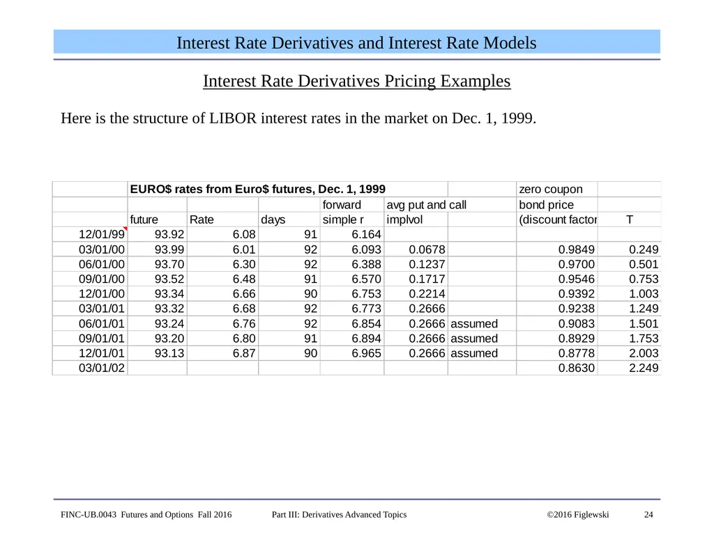
Here is the structure of LIBOR interest rates in the market on Dec. 1, 1999. FINC-UB.0043 Futures and Options Fall 2016 Part III: Derivatives Advanced Topics ©2016 Figlewski<br>
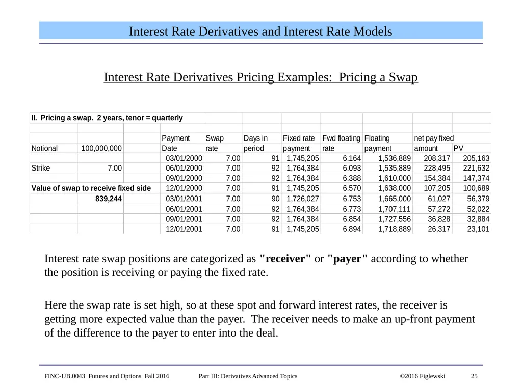
slide25. 25 Interest Rate Derivatives and Interest Rate Models Interest Rate Derivatives Pricing Examples: Pricing a Swap

Interest rate swap positions are categorized as "receiver" or "payer" according to whether the position is receiving or paying the fixed rate.

Here the swap rate is set high, so at these spot and forward interest rates, the receiver is getting more expected value than the payer. The receiver needs to make an up-front payment of the difference to the payer to enter into the deal. FINC-UB.0043 Futures and Options Fall 2016 Part III: Derivatives Advanced Topics ©2016 Figlewski<br>
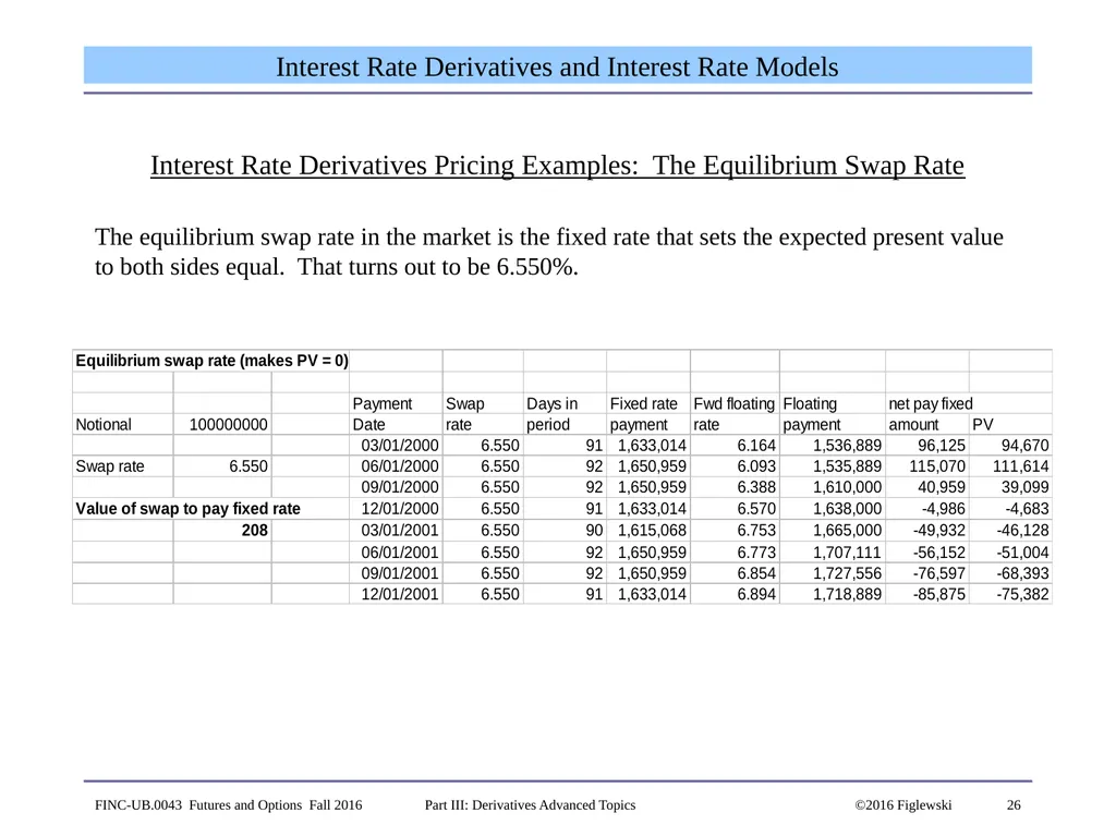
slide26. 26 Interest Rate Derivatives and Interest Rate Models Interest Rate Derivatives Pricing Examples: The Equilibrium Swap Rate

The equilibrium swap rate in the market is the fixed rate that sets the expected present value to both sides equal. That turns out to be 6.550%. FINC-UB.0043 Futures and Options Fall 2016 Part III: Derivatives Advanced Topics ©2016 Figlewski<br>
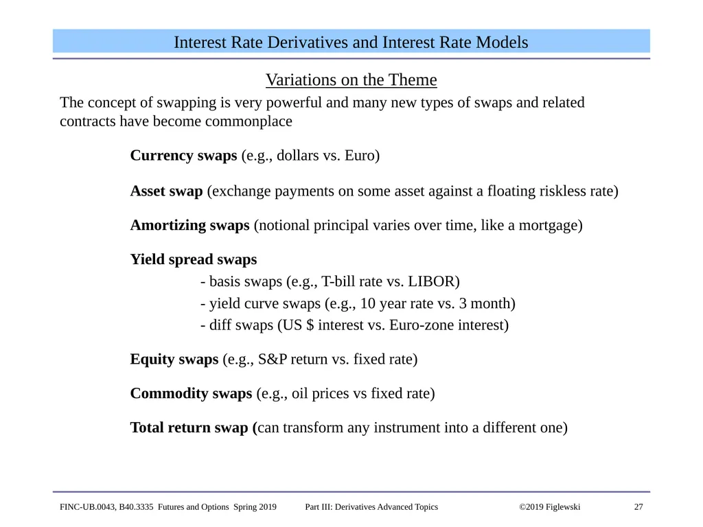
slide27. 27 Interest Rate Derivatives and Interest Rate Models Variations on the Theme
The concept of swapping is very powerful and many new types of swaps and related contracts have become commonplace

Currency swaps (e.g., dollars vs. Euro)

Asset swap (exchange payments on some asset against a floating riskless rate)

Amortizing swaps (notional principal varies over time, like a mortgage)

Yield spread swaps
- basis swaps (e.g., T-bill rate vs. LIBOR)
- yield curve swaps (e.g., 10 year rate vs. 3 month)
- diff swaps (US $ interest vs. Euro-zone interest)

Equity swaps (e.g., S&P return vs. fixed rate)

Commodity swaps (e.g., oil prices vs fixed rate)

Total return swap (can transform any instrument into a different one) FINC-UB.0043, B40.3335 Futures and Options Spring 2019 Part III: Derivatives Advanced Topics ©2019 Figlewski<br>
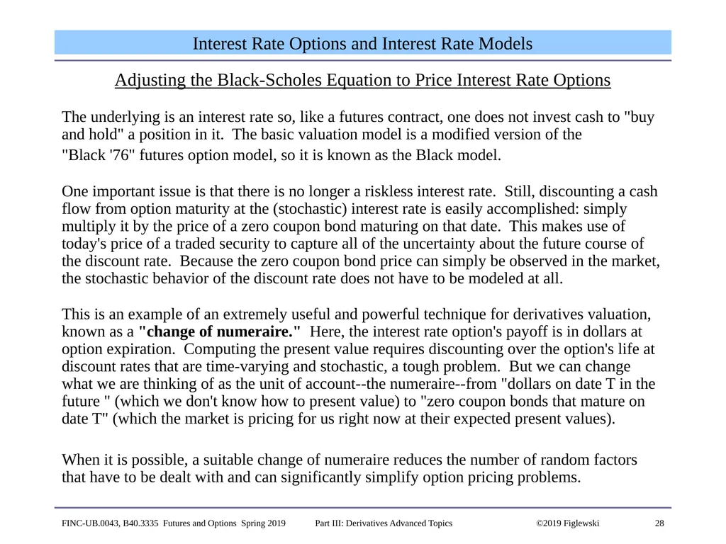
slide28. 28 Interest Rate Options and Interest Rate Models Adjusting the Black-Scholes Equation to Price Interest Rate Options

The underlying is an interest rate so, like a futures contract, one does not invest cash to "buy and hold" a position in it. The basic valuation model is a modified version of the
"Black '76" futures option model, so it is known as the Black model.

One important issue is that there is no longer a riskless interest rate. Still, discounting a cash flow from option maturity at the (stochastic) interest rate is easily accomplished: simply multiply it by the price of a zero coupon bond maturing on that date. This makes use of today's price of a traded security to capture all of the uncertainty about the future course of the discount rate. Because the zero coupon bond price can simply be observed in the market, the stochastic behavior of the discount rate does not have to be modeled at all.

This is an example of an extremely useful and powerful technique for derivatives valuation, known as a "change of numeraire." Here, the interest rate option's payoff is in dollars at option expiration. Computing the present value requires discounting over the option's life at discount rates that are time-varying and stochastic, a tough problem. But we can change what we are thinking of as the unit of account--the numeraire--from "dollars on date T in the future " (which we don't know how to present value) to "zero coupon bonds that mature on date T" (which the market is pricing for us right now at their expected present values).

When it is possible, a suitable change of numeraire reduces the number of random factors that have to be dealt with and can significantly simplify option pricing problems. FINC-UB.0043, B40.3335 Futures and Options Spring 2019 Part III: Derivatives Advanced Topics ©2019 Figlewski<br>
slide29. 29 Interest Rate Options and Interest Rate Models The Black Model for Interest Rate Options
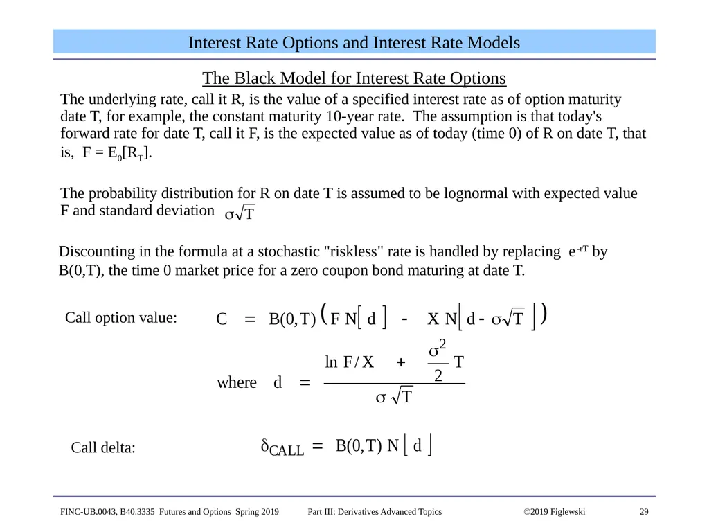
The underlying rate, call it R, is the value of a specified interest rate as of option maturity date T, for example, the constant maturity 10-year rate. The assumption is that today's forward rate for date T, call it F, is the expected value as of today (time 0) of R on date T, that is, F = E0[RT].

The probability distribution for R on date T is assumed to be lognormal with expected value F and standard deviation Call option value: Discounting in the formula at a stochastic "riskless" rate is handled by replacing e-rT by B(0,T), the time 0 market price for a zero coupon bond maturing at date T. Call delta: FINC-UB.0043, B40.3335 Futures and Options Spring 2019 Part III: Derivatives Advanced Topics ©2019 Figlewski<br>
slide30. 30 Interest Rate Options and Interest Rate Models The Black Model for Interest Rate Puts

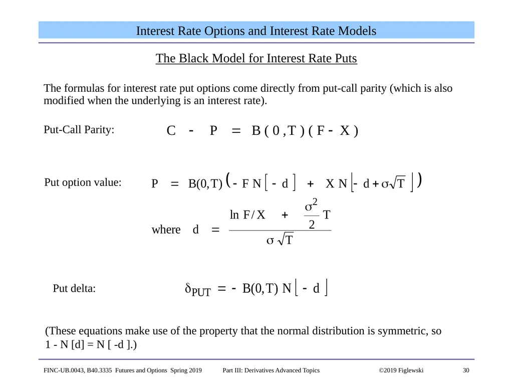
The formulas for interest rate put options come directly from put-call parity (which is also modified when the underlying is an interest rate).

Put-Call Parity: Put option value: Put delta: (These equations make use of the property that the normal distribution is symmetric, so
1 - N [d] = N [ -d ].) FINC-UB.0043, B40.3335 Futures and Options Spring 2019 Part III: Derivatives Advanced Topics ©2019 Figlewski<br>
slide31. 31 Interest Rate Derivatives and Interest Rate Models Interest Rate Derivatives Pricing Examples: Pricing a Caplet

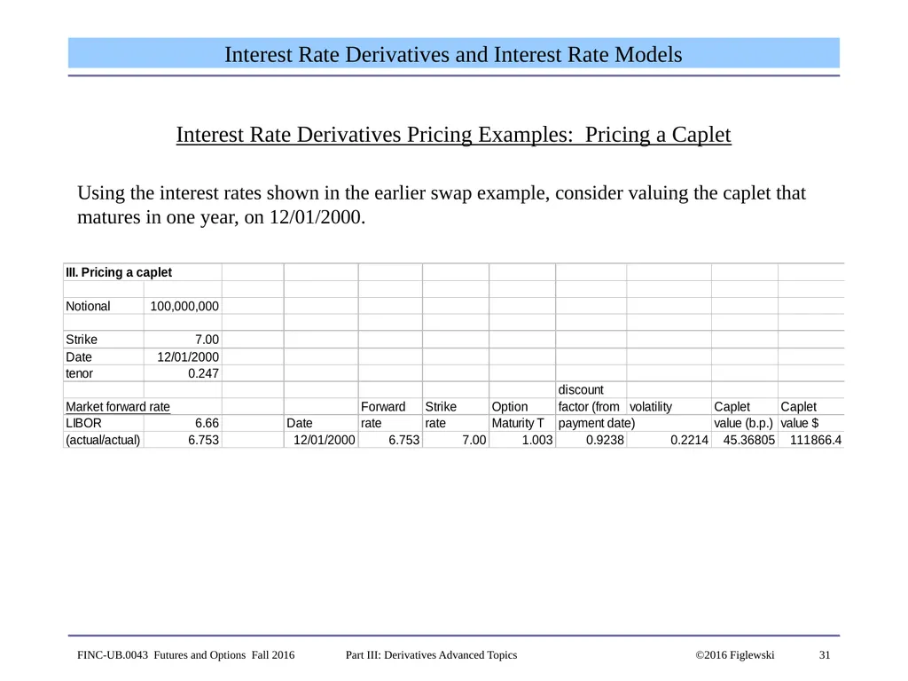
Using the interest rates shown in the earlier swap example, consider valuing the caplet that matures in one year, on 12/01/2000. FINC-UB.0043 Futures and Options Fall 2016 Part III: Derivatives Advanced Topics ©2016 Figlewski<br>
slide32. 32 Interest Rate Derivatives and Interest Rate Models Interest Rate Derivatives Pricing Examples: Pricing a Cap

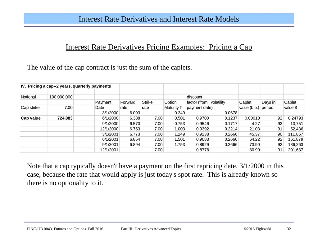
The value of the cap contract is just the sum of the caplets.

Note that a cap typically doesn't have a payment on the first repricing date, 3/1/2000 in this case, because the rate that would apply is just today's spot rate. This is already known so there is no optionality to it. FINC-UB.0043 Futures and Options Fall 2016 Part III: Derivatives Advanced Topics ©2016 Figlewski<br>
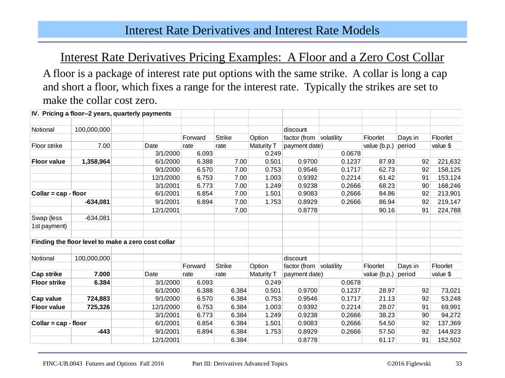
slide33. 33 Interest Rate Derivatives and Interest Rate Models Interest Rate Derivatives Pricing Examples: A Floor and a Zero Cost Collar
A floor is a package of interest rate put options with the same strike. A collar is long a cap and short a floor, which fixes a range for the interest rate. Typically the strikes are set to make the collar cost zero. FINC-UB.0043 Futures and Options Fall 2016 Part III: Derivatives Advanced Topics ©2016 Figlewski<br>
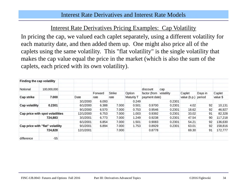
slide34. 34 Interest Rate Derivatives and Interest Rate Models Interest Rate Derivatives Pricing Examples: Cap Volatility
In pricing the cap, we valued each caplet separately, using a different volatility for each maturity date, and then added them up. One might also price all of the caplets using the same volatility. This "flat volatility" is the single volatility that makes the cap value equal the price in the market (which is also the sum of the caplets, each priced with its own volatility). FINC-UB.0043 Futures and Options Fall 2016 Part III: Derivatives Advanced Topics ©2016 Figlewski<br>
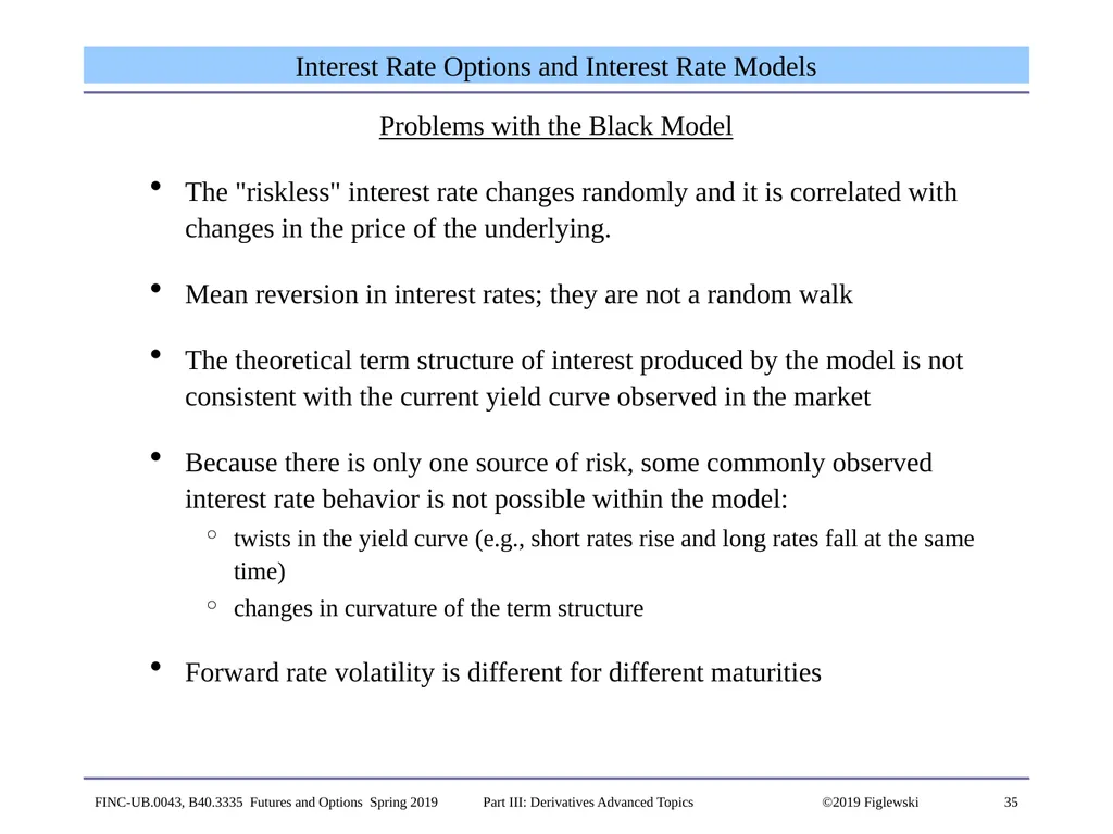
slide35. 35 Interest Rate Options and Interest Rate Models Problems with the Black Model

The "riskless" interest rate changes randomly and it is correlated with changes in the price of the underlying.

Mean reversion in interest rates; they are not a random walk

The theoretical term structure of interest produced by the model is not consistent with the current yield curve observed in the market

Because there is only one source of risk, some commonly observed interest rate behavior is not possible within the model:
twists in the yield curve (e.g., short rates rise and long rates fall at the same time)
changes in curvature of the term structure

Forward rate volatility is different for different maturities FINC-UB.0043, B40.3335 Futures and Options Spring 2019 Part III: Derivatives Advanced Topics ©2019 Figlewski<br>
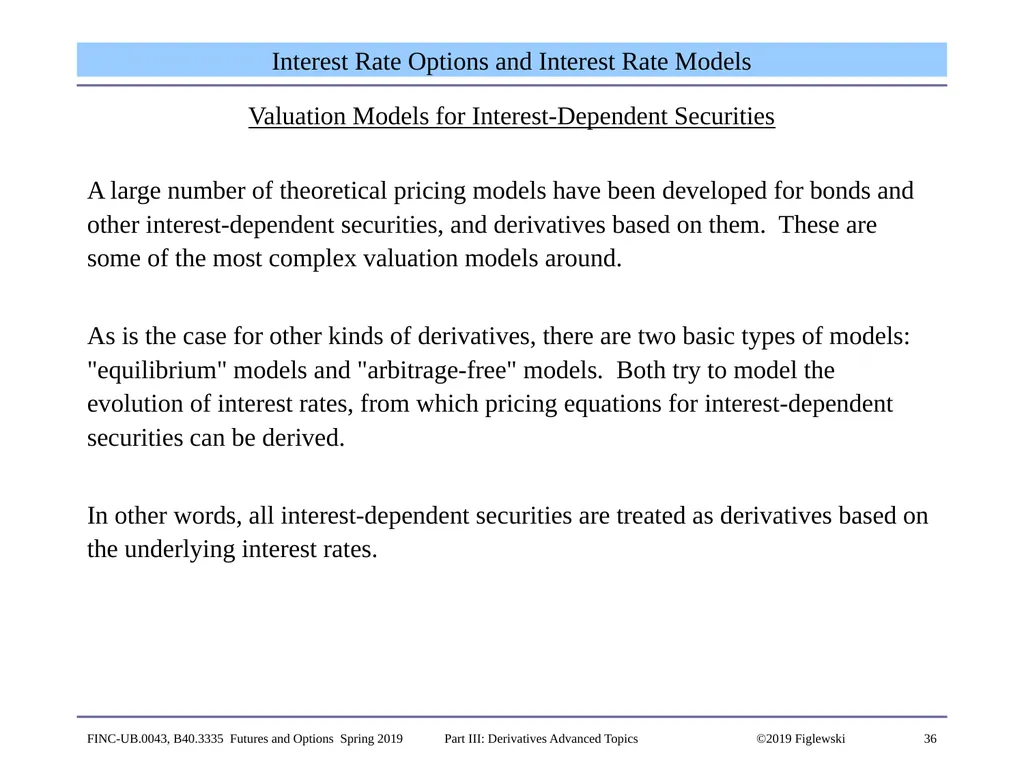
slide36. 36 Interest Rate Options and Interest Rate Models Valuation Models for Interest-Dependent Securities

A large number of theoretical pricing models have been developed for bonds and other interest-dependent securities, and derivatives based on them. These are some of the most complex valuation models around.

As is the case for other kinds of derivatives, there are two basic types of models: "equilibrium" models and "arbitrage-free" models. Both try to model the evolution of interest rates, from which pricing equations for interest-dependent securities can be derived.

In other words, all interest-dependent securities are treated as derivatives based on the underlying interest rates. FINC-UB.0043, B40.3335 Futures and Options Spring 2019 Part III: Derivatives Advanced Topics ©2019 Figlewski<br>
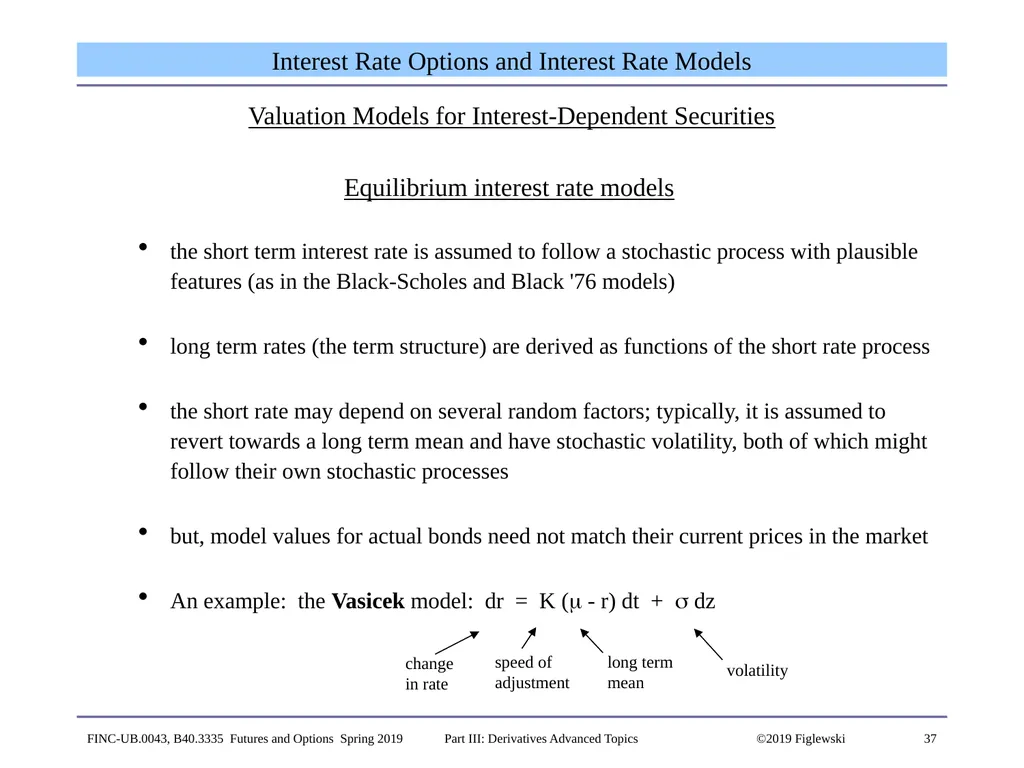
slide37. 37 Interest Rate Options and Interest Rate Models Valuation Models for Interest-Dependent Securities

Equilibrium interest rate models

the short term interest rate is assumed to follow a stochastic process with plausible features (as in the Black-Scholes and Black '76 models)

long term rates (the term structure) are derived as functions of the short rate process

the short rate may depend on several random factors; typically, it is assumed to revert towards a long term mean and have stochastic volatility, both of which might follow their own stochastic processes

but, model values for actual bonds need not match their current prices in the market

An example: the Vasicek model: dr = K ( - r) dt +  dz FINC-UB.0043, B40.3335 Futures and Options Spring 2019 Part III: Derivatives Advanced Topics ©2019 Figlewski<br>
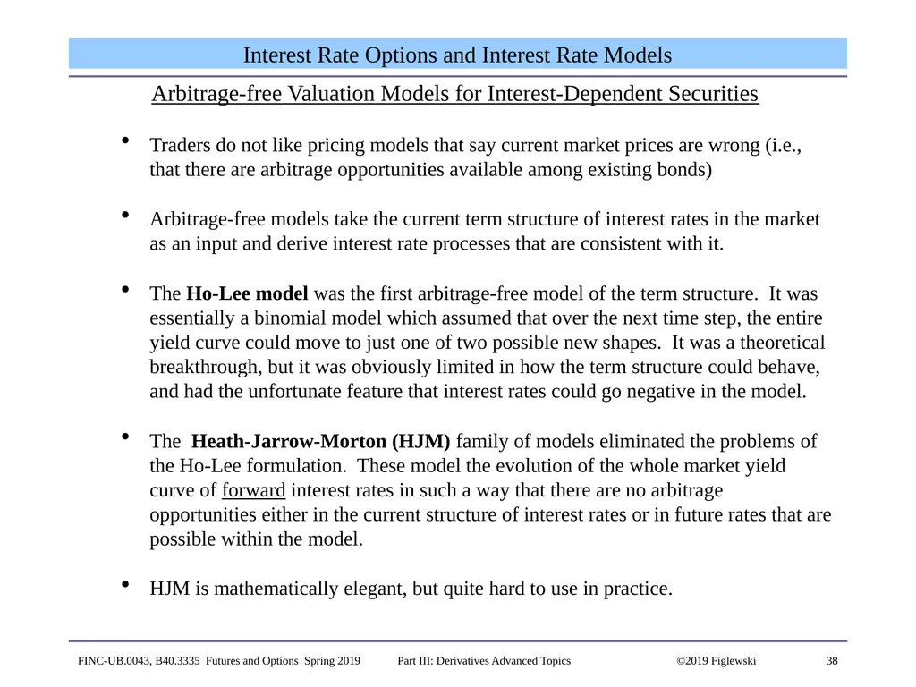
slide38. 38 Interest Rate Options and Interest Rate Models Arbitrage-free Valuation Models for Interest-Dependent Securities

Traders do not like pricing models that say current market prices are wrong (i.e., that there are arbitrage opportunities available among existing bonds)

Arbitrage-free models take the current term structure of interest rates in the market as an input and derive interest rate processes that are consistent with it.

The Ho-Lee model was the first arbitrage-free model of the term structure. It was essentially a binomial model which assumed that over the next time step, the entire yield curve could move to just one of two possible new shapes. It was a theoretical breakthrough, but it was obviously limited in how the term structure could behave, and had the unfortunate feature that interest rates could go negative in the model.

The Heath-Jarrow-Morton (HJM) family of models eliminated the problems of the Ho-Lee formulation. These model the evolution of the whole market yield curve of forward interest rates in such a way that there are no arbitrage opportunities either in the current structure of interest rates or in future rates that are possible within the model.

HJM is mathematically elegant, but quite hard to use in practice. FINC-UB.0043, B40.3335 Futures and Options Spring 2019 Part III: Derivatives Advanced Topics ©2019 Figlewski<br>
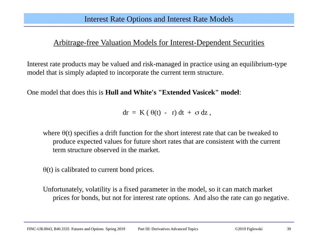
slide39. 39 Interest Rate Options and Interest Rate Models Arbitrage-free Valuation Models for Interest-Dependent Securities

Interest rate products may be valued and risk-managed in practice using an equilibrium-type model that is simply adapted to incorporate the current term structure.

One model that does this is Hull and White's "Extended Vasicek" model:

dr = K ( (t) - r) dt +  dz ,

where (t) specifies a drift function for the short interest rate that can be tweaked to produce expected values for future short rates that are consistent with the current term structure observed in the market.

(t) is calibrated to current bond prices.

Unfortunately, volatility is a fixed parameter in the model, so it can match market prices for bonds, but not for interest rate options. And also the rate can go negative. FINC-UB.0043, B40.3335 Futures and Options Spring 2019 Part III: Derivatives Advanced Topics ©2019 Figlewski<br>
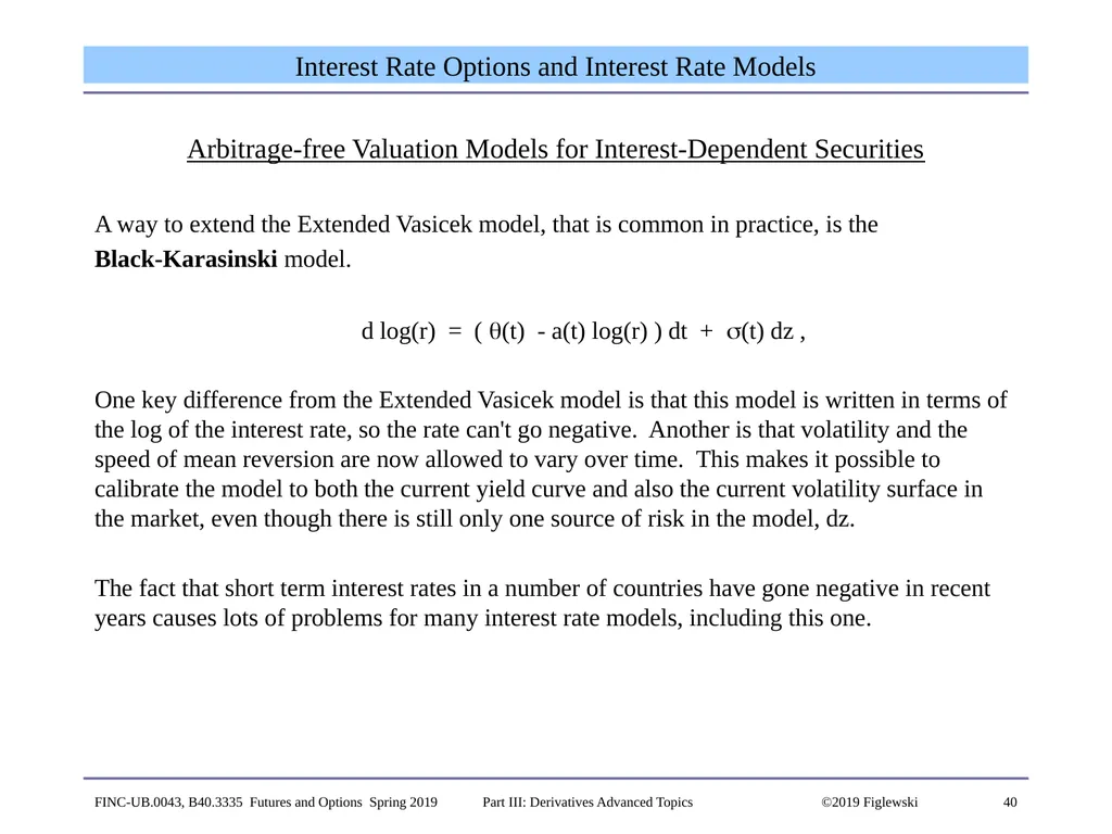
slide40. 40 Interest Rate Options and Interest Rate Models Arbitrage-free Valuation Models for Interest-Dependent Securities

A way to extend the Extended Vasicek model, that is common in practice, is the
Black-Karasinski model.

d log(r) = ( (t) - a(t) log(r) ) dt + (t) dz ,

One key difference from the Extended Vasicek model is that this model is written in terms of the log of the interest rate, so the rate can't go negative. Another is that volatility and the speed of mean reversion are now allowed to vary over time. This makes it possible to calibrate the model to both the current yield curve and also the current volatility surface in the market, even though there is still only one source of risk in the model, dz.

The fact that short term interest rates in a number of countries have gone negative in recent years causes lots of problems for many interest rate models, including this one. FINC-UB.0043, B40.3335 Futures and Options Spring 2019 Part III: Derivatives Advanced Topics ©2019 Figlewski<br>
slide41. 41 Interest Rate Options and Interest Rate Models Arbitrage-free Interest Rate Models: The Current State of the Art
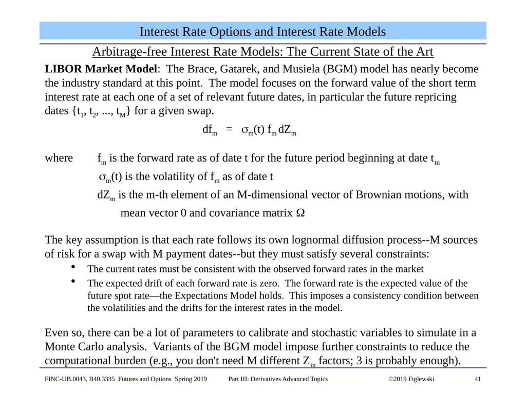
LIBOR Market Model: The Brace, Gatarek, and Musiela (BGM) model has nearly become the industry standard at this point. The model focuses on the forward value of the short term interest rate at each one of a set of relevant future dates, in particular the future repricing dates {t1, t2, ..., tM} for a given swap.
dfm = m(t) fm dZm

where fm is the forward rate as of date t for the future period beginning at date tm
m(t) is the volatility of fm as of date t
dZm is the m-th element of an M-dimensional vector of Brownian motions, with
mean vector 0 and covariance matrix 

The key assumption is that each rate follows its own lognormal diffusion process--M sources of risk for a swap with M payment dates--but they must satisfy several constraints:
The current rates must be consistent with the observed forward rates in the market
The expected drift of each forward rate is zero. The forward rate is the expected value of the future spot rate—the Expectations Model holds. This imposes a consistency condition between the volatilities and the drifts for the interest rates in the model.

Even so, there can be a lot of parameters to calibrate and stochastic variables to simulate in a Monte Carlo analysis. Variants of the BGM model impose further constraints to reduce the computational burden (e.g., you don't need M different Zm factors; 3 is probably enough). FINC-UB.0043, B40.3335 Futures and Options Spring 2019 Part III: Derivatives Advanced Topics ©2019 Figlewski<br>
slide42. 42 Bonds and Mortgages Bond Options
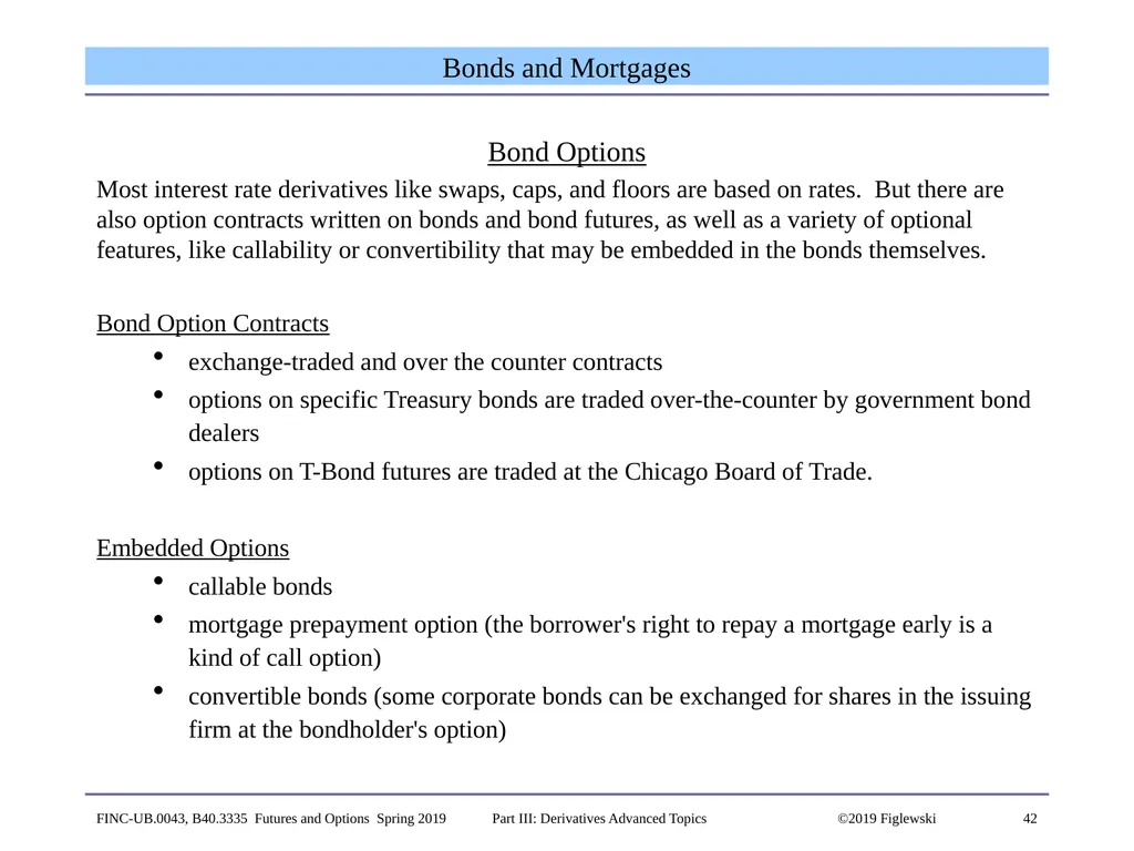
Most interest rate derivatives like swaps, caps, and floors are based on rates. But there are also option contracts written on bonds and bond futures, as well as a variety of optional features, like callability or convertibility that may be embedded in the bonds themselves.

Bond Option Contracts
exchange-traded and over the counter contracts
options on specific Treasury bonds are traded over-the-counter by government bond dealers
options on T-Bond futures are traded at the Chicago Board of Trade.

Embedded Options
callable bonds
mortgage prepayment option (the borrower's right to repay a mortgage early is a kind of call option)
convertible bonds (some corporate bonds can be exchanged for shares in the issuing firm at the bondholder's option) FINC-UB.0043, B40.3335 Futures and Options Spring 2019 Part III: Derivatives Advanced Topics ©2019 Figlewski<br>
slide43. 43 Callability in Bonds and Mortgages Callable Bonds
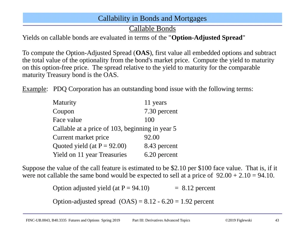
Yields on callable bonds are evaluated in terms of the "Option-Adjusted Spread"

To compute the Option-Adjusted Spread (OAS), first value all embedded options and subtract the total value of the optionality from the bond's market price. Compute the yield to maturity on this option-free price. The spread relative to the yield to maturity for the comparable maturity Treasury bond is the OAS.

Example: PDQ Corporation has an outstanding bond issue with the following terms:

Maturity 11 years
Coupon 7.30 percent
Face value 100
Callable at a price of 103, beginning in year 5
Current market price 92.00
Quoted yield (at P = 92.00) 8.43 percent
Yield on 11 year Treasuries 6.20 percent

Suppose the value of the call feature is estimated to be $2.10 per $100 face value. That is, if it were not callable the same bond would be expected to sell at a price of 92.00 + 2.10 = 94.10.

Option adjusted yield (at P = 94.10) = 8.12 percent

Option-adjusted spread (OAS) = 8.12 - 6.20 = 1.92 percent FINC-UB.0043, B40.3335 Futures and Options Spring 2019 Part III: Derivatives Advanced Topics ©2019 Figlewski<br>
slide44. 44 Mortgages Mortgages and Mortgage-Backed Securities

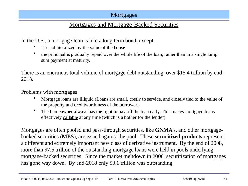
In the U.S., a mortgage loan is like a long term bond, except
it is collateralized by the value of the house
the principal is gradually repaid over the whole life of the loan, rather than in a single lump sum payment at maturity.

There is an enormous total volume of mortgage debt outstanding: over $15.4 trillion by end-2018.

Problems with mortgages
Mortgage loans are illiquid (Loans are small, costly to service, and closely tied to the value of the property and creditworthiness of the borrower.)
The homeowner always has the right to pay off the loan early. This makes mortgage loans effectively callable at any time (which is a bother for the lender).

Mortgages are often pooled and pass-through securities, like GNMA's, and other mortgage-backed securities (MBS), are issued against the pool. These securitized products represent a different and extremely important new class of derivative instrument. By the end of 2008, more than $7.5 trillion of the outstanding mortgage loans were held in pools underlying mortgage-backed securities. Since the market meltdown in 2008, securitization of mortgages has gone way down. By end-2018 only $3.1 trillion was outstanding. FINC-UB.0043, B40.3335 Futures and Options Spring 2019 Part III: Derivatives Advanced Topics ©2019 Figlewski<br>
slide45. 45 Mortgages Prepayment Risk

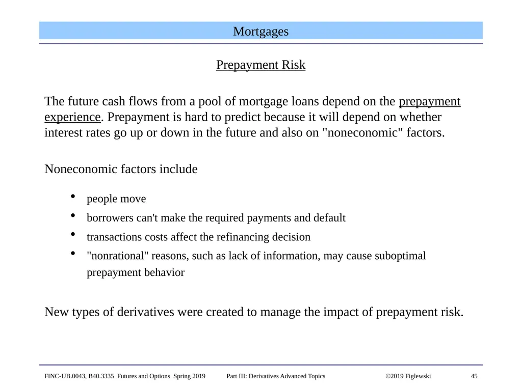
The future cash flows from a pool of mortgage loans depend on the prepayment experience. Prepayment is hard to predict because it will depend on whether interest rates go up or down in the future and also on "noneconomic" factors.

Noneconomic factors include

people move
borrowers can't make the required payments and default
transactions costs affect the refinancing decision
"nonrational" reasons, such as lack of information, may cause suboptimal prepayment behavior

New types of derivatives were created to manage the impact of prepayment risk. FINC-UB.0043, B40.3335 Futures and Options Spring 2019 Part III: Derivatives Advanced Topics ©2019 Figlewski<br>
slide46. 46 Mortgages Prepayment Risk and Valuation

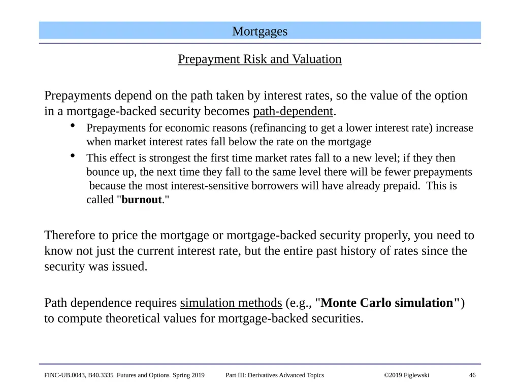
Prepayments depend on the path taken by interest rates, so the value of the option in a mortgage-backed security becomes path-dependent.
Prepayments for economic reasons (refinancing to get a lower interest rate) increase when market interest rates fall below the rate on the mortgage
This effect is strongest the first time market rates fall to a new level; if they then bounce up, the next time they fall to the same level there will be fewer prepayments because the most interest-sensitive borrowers will have already prepaid. This is called "burnout."

Therefore to price the mortgage or mortgage-backed security properly, you need to know not just the current interest rate, but the entire past history of rates since the security was issued.

Path dependence requires simulation methods (e.g., "Monte Carlo simulation") to compute theoretical values for mortgage-backed securities. FINC-UB.0043, B40.3335 Futures and Options Spring 2019 Part III: Derivatives Advanced Topics ©2019 Figlewski<br>
slide47. 47 Mortgage-Backed Securities Mortgage Loans

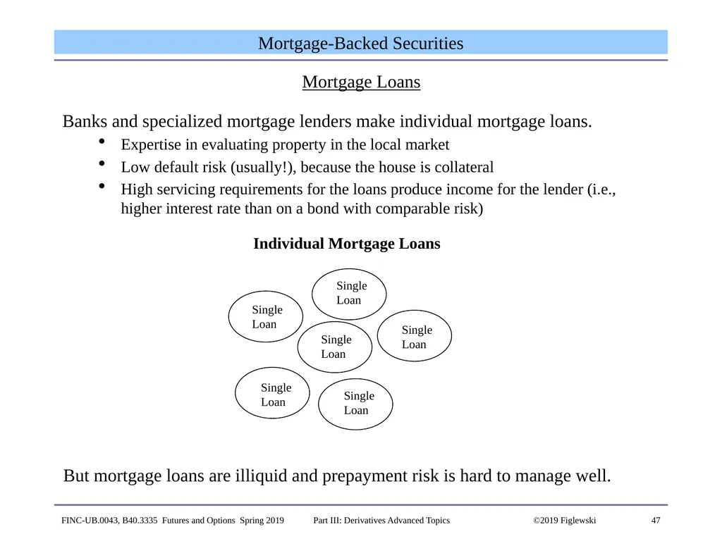
Banks and specialized mortgage lenders make individual mortgage loans.
Expertise in evaluating property in the local market
Low default risk (usually!), because the house is collateral
High servicing requirements for the loans produce income for the lender (i.e., higher interest rate than on a bond with comparable risk) But mortgage loans are illiquid and prepayment risk is hard to manage well. FINC-UB.0043, B40.3335 Futures and Options Spring 2019 Part III: Derivatives Advanced Topics ©2019 Figlewski<br>
slide48. 48 Mortgage-Backed Securities Mortgage Pass-Throughs

Following the "Credit Crunch" of 1966, the Government National Mortgage Association (GNMA, known as "Ginnie Mae") was created in 1970 to provide a new mechanism for financing mortgage loans.
The new financing idea is known as securitization.
The new financial instrument was the mortgage pass-through security.

Mortgage lenders "originate" loans (they set them up). Once a number of similar mortgage loans have been made, they are bundled together into a mortgage pool and GNMA pass-through securities are issued and sold in the securities market.

A mortgage pass-through is similar to a bond. Each month, as the homeowners make their mortgage payments,
the originating bank retains a fee for servicing the loan
the rest of the funds are passed through to the holders of the pass-through securities
to be eligible for inclusion in a GNMA pool, a mortgage loan must be insured by the government (e.g., the Veteran's Administration). There is no risk to the lender from a borrower default.
prepayments of principal from loans paid off early by borrowers or from government payoffs of defaulted loans are also passed through. This makes monthly cash flow irregular and hard to predict. FINC-UB.0043, B40.3335 Futures and Options Spring 2019 Part III: Derivatives Advanced Topics ©2019 Figlewski<br>
slide49. 49 Mortgage Pool Mortgage-Backed Securities Mortgage Pass-Throughs

The GNMA pass-through revolutionized the mortgage market. Funding of home loans no longer depended on the ability of savings banks and S&Ls (savings and loan institutions) to attract deposits: funds could be obtained as needed in the bond market.

But prepayments still create substantial risk for the investor.
Cash flows are less predictable than with regular bonds
Prepayments increase when interest rates at which the funds can be reinvested are low, to the disadvantage of the lender Single
Loan Single
Loan Single
Loan Single
Loan Single
Loan Single
Loan pass-through security Cash flows from the mortgage pool are allocated proportionally to the pass-through securities pass-through security pass-through security pass-through security FINC-UB.0043, B40.3335 Futures and Options Spring 2019 Part III: Derivatives Advanced Topics ©2019 Figlewski<br>
slide50. 50 Mortgage-Backed Securities Collateralized Mortgage Obligations (CMOs)
Before long further innovations were introduced. More complex structures called CMOs were introduced, with different "tranches" (French for "slice") of securities.

Each month when the homeowners make their mortgage payments
holders of the "A" tranche get their promised payments first--these are extremely predictable
then "B" tranche holders are paid from the remaining funds, and so on
uncertainty in the total cash flows from the pool due to prepayment risk is concentrated in the lower priority classes Cash flows from mortgage pool are allocated to different priority classes (tranches) of mortgage-backed securities "toxic waste" FINC-UB.0043, B40.3335 Futures and Options Spring 2019 Part III: Derivatives Advanced Topics ©2019 Figlewski<br>
slide51. 51 Mortgage-Backed Securities Pricing MBS using Monte Carlo Simulation

The payoffs on basic forwards, futures and European options depend on the price of the underlying asset at the expiration of the contract. It doesn't matter how the price gets from today's value to the final value. The payoff is independent of the path.

American options are different because you might want to exercise early, depending on where the asset price is on one or more dates before expiration. The option is path-dependent, but only in a limited way. At each date you can decide whether to exercise or not, but that decision will depend only on how the price might evolve from that date forward. It doesn't matter how it got to its present level.

Mortgages and mortgage-backed securities are path-dependent in a more complicated way. The timing and amounts of their payoffs are a function of the prepayment experience on the underlying mortgage loans. It does matter what path interest rates have followed in getting to today's level. That makes it impossible to price MBS with the standard backward recursion technology we have considered so far. FINC-UB.0043, B40.3335 Futures and Options Spring 2019 Part III: Derivatives Advanced Topics ©2019 Figlewski<br>
slide52. 52 Mortgage-Backed Securities Pricing MBS using Monte Carlo Simulation, p.2

Consider an MBS that is backed by a pool of mortgage loans with a 6% fixed interest rate. We may know that the rate in the market is 6.5% today, but that's not enough to value the MBS. Its future cash flows will be affected by how many of the underlying mortgages have already prepaid, and that depends on how interest rates have moved before now.

If the rate has remained above 6% since the pool was formed, there may have been comparatively few prepayments. But if rates have dropped to 4% and then gone back up to today's 6.5%, many of the original borrowers will have prepaid their 6% loans and refinanced at the lower rates. The number of mortgages left in the pool will be much fewer.

Path-dependent securities like MBS have to be priced approximately, by Monte Carlo simulation. FINC-UB.0043, B40.3335 Futures and Options Spring 2019 Part III: Derivatives Advanced Topics ©2019 Figlewski<br>
slide53. 53 Mortgage-Backed Securities Pricing MBS using Monte Carlo Simulation, p.3
Monte Carlo simulation starts with a model, like one of the interest models we have looked at, for how the underlying risk factor(s) behave.

Interest rate model (Vasicek): dr =  (  - r ) dt +  dz

Discretized for interval Δt:

A possible path for future interest rates {r1, r2, ..., rT} is simulated by drawing random numbers from a standard normal distribution (or whatever distribution one thinks is most appropriate) and plugging them into the equations for the stochastic {zt} terms. Once a full path of rates from the present to maturity is generated, a prepayment model is used to compute expected prepayments from the pool along that interest rate path.

Vi = V({r1, r2, ..., rT}i , prepayments)

The present value of the simulated cash flows along the ith simulated interest rate path gives one observation, Vi , for the possible value of the MBS consistent with the interest rate model and the assumed prepayment behavior. FINC-UB.0043, B40.3335 Futures and Options Spring 2019 Part III: Derivatives Advanced Topics ©2019 Figlewski<br>
slide54. 54 Mortgage-Backed Securities Pricing MBS using Monte Carlo Simulation, p.4

This process is then repeated, maybe N = 100,000 times. In the end, one has 100,000 possible outcomes that are consistent with the interest rate process and the prepayment model. These are used to compute the mean, standard deviation, and other necessary statistics for the returns distribution, from which the MBS fair value V and risk parameters are obtained.
V = mean( {Vi, i = 1,...,N} )

Monte Carlo simulation is heavily used for solving models in:
weather forecasting
nuclear weapons design
financial derivatives FINC-UB.0043, B40.3335 Futures and Options Spring 2019 Part III: Derivatives Advanced Topics ©2019 Figlewski<br>
slide55. 55 Credit Risk: Default as an Option and Credit Derivatives Up to this point, our focus has been on hedging and managing exposure to the risk of adverse fluctuations in the market values of our assets or liabilities. But for many financial institutions like banks, the risk that worries them most is not that the present value of the repayments on a loan will go down, but that the borrower will not repay the loan at all, i.e., credit risk.

An early insight from modern option valuation technology was that securities issued by a corporation, like stocks and bonds, are actually derivatives whose values are derived from the value of the underlying firm. Option pricing theory can help us understand the risk of bankruptcy embedded in corporate securities. (Who thought of this? Robert Merton, of course, in the 1970s!)

Thinking of the stock as an option on the assets of the firm can help us value risky debt and also clarifies how limited liability gives shareholders the incentive to increase risk exposure at the firm level. The current "structural" and "reduced form" approaches to evaluating credit risk have developed from this insight.

Finally we take a look at two important new types of derivative instruments that have been developed specifically for managing credit risk: credit default swaps (CDS) and collateralized debt obligations (CDOs). FINC-UB.0043, B40.3335 Futures and Options Spring 2019 Part III: Derivatives Advanced Topics ©2019 Figlewski<br>
slide56. 56 Credit Risk: Default as an Option and Credit Derivatives Models of Default Risk

There are two basic derivatives-related approaches to analyzing and valuing risky debt (i.e. debt with a risk of default): "Structural" models (based on ideas first published in a paper by Merton in 1974), and "Reduced Form" models.

Structural Models

The true underlying asset is the whole firm, with current value Vt.

Vt follows a Black-Scholes type diffusion process

Bonds with face value F, maturing at date T, are paid off if VT > F

If VT < F, the firm defaults and the bondholders take over the firm (they get VT)

This makes equity a kind of call option on the underlying firm value V FINC-UB.0043, B40.3335 Futures and Options Spring 2019 Part III: Derivatives Advanced Topics ©2019 Figlewski<br>
slide57. 57 Credit Risk: Default as an Option and Credit Derivatives The Structural Approach: Corporate Securities as Options on the Firm
 The ability to default is an option

Consider a firm with a very basic capital structure. It has issued stock and a single zero coupon bond.

Let V = Value of the entire firm.
F = Face value of bonds to be paid off at date T.

V is assumed to follow the standard lognormal diffusion process Consider the payoffs on the different securities on date T as a function of the firm value on that date, VT. FINC-UB.0043, B40.3335 Futures and Options Spring 2019 Part III: Derivatives Advanced Topics ©2019 Figlewski<br>
slide58. 58 Credit Risk: Default as an Option and Credit Derivatives Default in a Structural Model FINC-UB.0043, B40.3335 Futures and Options Spring 2019 Part III: Derivatives Advanced Topics ©2019 Figlewski<br>
slide59. 59 Credit Risk: Default as an Option and Credit Derivatives Security Payoffs at Bond Maturity, Date T

VT < F F < VT

1. STOCK 0 VT - F
  Firm is bankrupt Firm is solvent.
Bonds are paid in full.

2. BONDS VT F
  Firm is bankrupt. Firm is solvent.
Assets distributed Bonds are paid
to bondholders off at face value.

Here it looks like the bondholders own the firm but the stockholders can call it away from them if the date T firm value is high.

This is kind of a strange way to think about it. We normally think the shareholders own the firm, but can turn it over to the creditors at date T instead of paying off the bonds. FINC-UB.0043, B40.3335 Futures and Options Spring 2019 Part III: Derivatives Advanced Topics ©2019 Figlewski<br>
slide60. 60 Credit Risk: Default as an Option and Credit Derivatives Another Way to Think about Security Payoffs at Date T Bond Maturity
(yet another example of put-call parity!)
The bondholders have riskless bonds, but have written a put option to the stockholders:

VT < F F < VT

1. STOCK Firm is "put" to VT - F
  bondholders instead
of paying F Bonds are paid in full.

2. BONDS
Default-free bond F F
  + Firm is solvent
Short a put option
on the firm value V - (F - VT ) Short put is worthless
with strike price F
VT F FINC-UB.0043, B40.3335 Futures and Options Spring 2019 Part III: Derivatives Advanced Topics ©2019 Figlewski<br>
slide61. 61 Credit Risk: Default as an Option and Credit Derivatives Implications of Modeling Stock and Bonds as Contingent Claims

The stock is an option on the firm and option value is enhanced by higher volatility.
The shareholders have an incentive to increase firm risk. (This shifts value from the bondholders to the stockholders.)
One way to increase risk is to distribute firm assets to the shareholders (paying dividends); this is typically restricted by covenants in the bond indenture agreement.
but sometimes other opportunities arise to transfer firm value from the bondholders to the stockholders, e.g., RJR Nabisco in the late 1980s (see the book and movie "Barbarians at the Gates")

This approach is one of the major ways of addressing credit risk on bonds within the standard contingent claims valuation paradigm.
KMV (now Moody's KMV) is major firm currently doing credit analysis based largely on the structural framework. FINC-UB.0043, B40.3335 Futures and Options Spring 2019 Part III: Derivatives Advanced Topics ©2019 Figlewski<br>
slide62. 62 Credit Risk: Default as an Option and Credit Derivatives Problems with Structural Models of Default Risk

Firm value is hard to determine for real-world firms

Actual debt contracts are much more complicated than what Merton models
"bonds" are coupon debt, with many small periodic payments before maturity, call provisions and other special features
firms may have issued multiple classes of debt with different maturities and other terms (senior debt, junior debt, bank loans, lines of credit, commercial paper, etc., etc.)
priority rules for who gets paid off first are often violated in real world bankruptcy proceedings
it is difficult to model the firm's optimal default strategy

The structural approach is little help in valuing many popular kinds of credit derivatives whose payoffs are tied to a change in bond rating or yield spread, not to actual default FINC-UB.0043, B40.3335 Futures and Options Spring 2019 Part III: Derivatives Advanced Topics ©2019 Figlewski<br>
slide63. 63 Credit Risk: Default as an Option and Credit Derivatives Reduced Form Models of Default Risk

The other major class of default models does not try to look carefully inside the corporation, but just focuses on overall probabilities. These are known as "reduced form" models.

Default is a random event, like a lightning strike, that could happen to any firm at any time.

Default is modeled as a Poisson process (a probability model for infrequently occurring big events; almost the exact opposite of a diffusion process).

Default intensity (the probability of a default within a given span of time) can be modeled as exogenous, or as a function of firm value and other variables.

Payoff on bonds if default occurs is not VT, but some exogenously specified recovery rate (empirical recovery rates are quite variable, but average around 40 - 50%).

Invented about 1800 by the French mathematician Siméon Denis Poisson. FINC-UB.0043, B40.3335 Futures and Options Spring 2019 Part III: Derivatives Advanced Topics ©2019 Figlewski<br>
slide64. 64 Credit Risk: Default as an Option and Credit Derivatives Moody's KMVHistorical Credit Ratings Transition Matrix

Source: Moodys KMV. "Default and Recovery Rates of Corporate Bond Issuers, 1920-2015." FINC-UB.0043, B40.3335 Futures and Options Spring 2019 Part III: Derivatives Advanced Topics ©2019 Figlewski<br>
slide65. 65 Credit Risk: Default as an Option and Credit Derivatives Beginning in the mid-1990s, derivatives based on credit risk began to appear. The simplest is the credit default swap (CDS), a derivative contract that functions very much like an insurance policy against default by a bond issuer.

The collateralized debt obligation (CDO) uses securitization and tranching, as in mortgage-backed securities, to reallocate the incidence of the default risk in a portfolio of risky bonds. An MBS concentrates prepayment risk into a small fraction of the new securities, leaving the rest with virtually none. In the same way, a CDO concentrates default risk into a small fraction of the CDO tranche securities, leaving most of the tranches at AAA quality or above, even when the underlying bonds in the pool are much riskier.

Unfortunately, valuation models for credit derivatives are complicated and hard to test empirically because defaults are such rare events (luckily!). Pricing in the real world does not seem to be entirely consistent with the theoretical models. FINC-UB.0043, B40.3335 Futures and Options Spring 2019 Part III: Derivatives Advanced Topics ©2019 Figlewski<br>
slide66. 66 Credit Risk: Default as an Option and Credit Derivatives Credit Default Swaps

A CDS is a derivative contract based on default risk. Like a futures contract, a CDS transfers risk from the owner of the risky security to the derivatives counterparty.

How it works (originally):
Counterparty A (the protection buyer) commits to make regular premium payments to Counterparty B. The rate is S basis points per year, applied to a notional face value F.

Counterparty B (the protection seller) commits to make the following payments to A:
If there is no default by the "reference entity" (the bond issuer) before the CDS expires, B pays nothing.
If the reference entity defaults, B must compensate A's loss. Either
A delivers bonds issued by the defaulting entity, and B pays A their face value F, or
B pays a cash amount to A, equal to the difference between the post-default price of the bonds and face value F. The price is determined in a special auction 1 month after the credit event. FINC-UB.0043, B40.3335 Futures and Options Spring 2019 Part III: Derivatives Advanced Topics ©2019 Figlewski<br>
slide67. 67 Credit Risk: Default as an Option and Credit Derivatives Credit Default Swaps

This setup was originally designed for an OTC market. Each deal had its own CDS spread S and maturity date. Maturities were standard, with 5 years the most common, then 10 years, but a 5-year contract matured 5 years after the date it was issued.

Both of these features made every CDS contract nonstandard, and therefore greatly limited its liquidity.

Market conventions were changed in 2009:
The premium payments are now standardized, so most CDS pay 100 basis points annually (very high risk CDS pay 500 b.p.), and an upfront payment adjusts for the precise level of default risk.
If equilibrium CDS spread S for a particular issuer would be below 100 b.p., the protection seller would be receiving too much premium, so the seller pays the buyer the fair value of the difference up front.
If equilibrium S would be above 100 b.p., the buyer pays the seller up front.
Maturity dates are also standardized to be every 6 months. Contract maturities for 5-year CDS on their issue date are now between 4 3/4 and 5 1/4 years.

These changes were big improvements to liquidity in the secondary market for CDS. FINC-UB.0043, B40.3335 Futures and Options Spring 2019 Part III: Derivatives Advanced Topics ©2019 Figlewski<br>
slide68. 68 Credit Risk: Default as an Option and Credit Derivatives An Extremely Important Innovation: The Credit Default Swap

For many institutional investors, market price risk is much less important than risk of default. The CDS is a way to buy (or sell) insurance against default.
The protection buyer pays a regular quarterly premium to the protection seller. If there is a default, the protection seller must pay the protection buyer. The amount of compensation that is determined at a special auction of the defaulted bonds about a month later. CDS premiums;
plus defaulted bonds, if any Credit default swap Total Alpha Fund
buys protection
on bonds
issued by
XYZ Corp. FINC-UB.0043, B40.3335 Futures and Options Spring 2019 Part III: Derivatives Advanced Topics ©2019 Figlewski<br>
slide69. 69 Credit Risk: Default as an Option and Credit Derivatives An Extremely Important Innovation: The Credit Default Swap
In the previous example, the Total Alpha Fund bought protection to eliminate the default risk on XYZ Corp. bonds, to produce a portfolio with credit quality better than AAA.

Alternatively, Total Alpha could hold a portfolio of Treasury bonds and sell protection on XYZ. It would then receive regular premium payments from its counterparty, but would bear the risk of loss if a default occurs. This way Total Alpha earns the return, including risk premium, on risky XYZ bonds (and bears the default risk) without actually owning them. Credit default swap FINC-UB.0043, B40.3335 Futures and Options Spring 2019 Part III: Derivatives Advanced Topics ©2019 Figlewski<br>
slide70. 70 Credit Risk: Default as an Option and Credit Derivatives CDS Pricing
Originally, the equilibrium CDS spread was the value of the spread S that set the (risk neutral!) expected values of the "premium leg" and the "protection leg" equal. For a T period CDS,

Let pi = probability of default in period i, for a bond that starts at time 0
Di = the discount factor for premium payment i
i = the length of the payment period
R = fraction of face value recovered in case of default
V0 = upfront payment by protection buyer (negative if seller pays upfront)

Premium Leg
E[PV(future stream of premiums)] =

Protection Leg
E[PV(payoff in case of default)] =

Under the new procedures: S is always set at 100 (or 500). The two legs will not have the same value. The difference between them is the upfront payment that will be needed. probability of no default prior to period i FINC-UB.0043, B40.3335 Futures and Options Spring 2019 Part III: Derivatives Advanced Topics ©2019 Figlewski<br>
slide71. 71 Credit Risk: Default as an Option and Credit Derivatives The Equilibrium CDS Spread S versus the Credit Spread in Bonds

The equilibrium CDS spread should be close to the credit spread on the firm's bonds in the bond market relative to Treasuries. But the spreads are not equal in practice, and there are some practical reasons why they should not be equal.

There is an option of which bonds to deliver against the CDS (any bonds issued by the defaulting firm—the "reference entity"– may be delivered

At the time of default, accrued premium since the previous payment date must be paid by the protection buyer, but the holder of the defaulted bonds doesn't get any accrued interest

Both corporate bonds and CDS are subject to market noise, which reduces measured correlation between them (corporate bonds are pretty illiquid) FINC-UB.0043, B40.3335 Futures and Options Spring 2019 Part III: Derivatives Advanced Topics ©2019 Figlewski<br>
slide72. 72 Credit Risk: Default as an Option and Credit Derivatives The Recovery Rate Assumption

The recovery rate assumption has a very significant impact on CDS pricing.

The recovery rate is hard to predict accurately. It is commonly simply set to the long run average recovery fraction, approximately 40%.

Average recovery rates have been found to vary over a wide range across different defaults and over time

recoveries are negatively correlated with (physical) default probabilities (the more likely default is, the less will probably be recovered if default happens) FINC-UB.0043, B40.3335 Futures and Options Spring 2019 Part III: Derivatives Advanced Topics ©2019 Figlewski<br>
slide73. 73 Credit Risk: Default as an Option and Credit Derivatives Collateralized Debt Obligation (CDO)
CDS (Credit Default Swaps) are like a combination of futures and insurance. The primary purpose is to transfer exposure to risk

CDOs (Collateralized Debt Obligations) are derivatives created through securitization, like mortgage-backed securities. The primary purpose is to repackage risk exposure.

A CDO is a securitization of debt securities

risky bonds, or loans, are pooled and new securities similar to CMOs are issued, with different priorities over the cash flows
CDOs can concentrate the default risk of the underlying bonds into a few high-risk securities, leaving the others essentially risk free
"synthetic CDOs" are pools not of risky bonds, but of CDS
one of the most important properties of the pool is the correlation in default risk across issuers (which determines the risk that a lot of bonds will go bad together)

Originally, most mortgages in the pools supporting mortgage pass-throughs and CMOs were guaranteed by the government, so there was no credit risk. In the years following 2000, a large volume of CMOs based on pools of "subprime" and "Alt-A" mortgage loans were created. These are not guaranteed, so the CMOs were exposed to both prepayment risk and default risk. In a number of cases the underlying mortgages were so bad that the tranching failed to protect the senior tranches. FINC-UB.0043, B40.3335 Futures and Options Spring 2019 Part III: Derivatives Advanced Topics ©2019 Figlewski<br>
slide74. 74 Credit Risk: Default as an Option and Credit Derivatives Collateralized Debt Obligations

Securitization and tranching used in creating mortgage-backed securities can be applied to other kinds of loans (student loans, auto loans, credit card receivables, etc., etc.).

Some of the most exciting new securitized instruments are Collateralized Debt Obligations and Collateralized Loan Obligations (CLOs)
pools of credit-risky bonds or loans are bundled together ("cash flow CDO")
a common alternative structure is the "synthetic CDO," in which the pool of securities exposed to credit risk consists of Credit Default Swaps, rather than actual bonds FINC-UB.0043, B40.3335 Futures and Options Spring 2019 Part III: Derivatives Advanced Topics ©2019 Figlewski<br>
slide75. 75 Credit Risk: Default as an Option and Credit Derivatives Allocation of Default Losses in CDOs

In a CDO, default losses are allocated first to the lowest tranche

the "senior" and "super-senior" tranches are typically more than 80% of the total principal value
these can be rated AAA, even though the underlying bonds or loans are rated much lower. FINC-UB.0043, B40.3335 Futures and Options Spring 2019 Part III: Derivatives Advanced Topics ©2019 Figlewski<br>
slide76. 76 Credit Risk: Default as an Option and Credit Derivatives Allocation of Default Losses in CDOs

The price for the equity tranche is quoted differently from the other tranches in the market because it has a relatively high probability of being completely wiped out before the pool matures FINC-UB.0043, B40.3335 Futures and Options Spring 2019 Part III: Derivatives Advanced Topics ©2019 Figlewski<br>
slide77. 77 Credit Risk: Default as an Option and Credit Derivatives CDOs
The essential features of a CDO are securitization and tranching.

Typical structure

Just like with a CMO, the cash flows into the portfolio, either from bond coupon and principal payments (or from CDS premiums received in a synthetic structure) are passed through and allocated to the tranches, in a "waterfall" pattern.

If there is a default, the principal backing the equity tranche is reduced by the amount of the loss. All default losses are allocated to the equity tranche until the total loss is greater than 3% of the initial principal and the tranche is totally wiped out. Any defaults after that will be borne by the mezzanine tranche, until 7% of the face value has been wiped out. (Note that because there are recoveries, this would mean that a lot more than 7% of the bonds have defaulted.)

The super senior tranche is insulated against all defaults on the portfolio that do not total more than 12% of initial principal. This is extremely unlikely unless defaults are highly correlated. FINC-UB.0043, B40.3335 Futures and Options Spring 2019 Part III: Derivatives Advanced Topics ©2019 Figlewski<br>
slide78. 78 Credit Risk: Default as an Option and Credit Derivatives Correlation and CDO Valuation

One of the major determinants of default risk exposure in a CDO is correlation in defaults.

A simple example:
The "portfolio" = 50% in bonds from issuer A and 50% in bonds from issuer B.
Both A and B have 10% probability of defaulting within the next year.
There are two CDO tranches issued, each covering 50% of face value.

The equity tranche (0 - 50%) takes the first loss. It has a total loss if either A or B (or both) defaults.

The senior tranche only takes the second loss, so there is no loss to the senior tranche unless both A and B default. FINC-UB.0043, B40.3335 Futures and Options Spring 2019 Part III: Derivatives Advanced Topics ©2019 Figlewski<br>
slide79. 79 Credit Risk: Default as an Option and Credit Derivatives Correlation and CDO Valuation, p.2
Impact of correlation

If  = 0, defaults are independent
prob(loss to equity tranche) =
p(A) + p(B) - p(A and B) = 19%.
prob(loss to senior tranche) = p(A)  p(B) = 1%.

If   1.0, defaults for both A and B occur together
prob(loss to equity tranche) = p(A) = p(B) = 10%.
prob(loss to senior tranche) = p(A) = p(B) = 10%.

The basic result: Higher default correlation increases
the value of the equity tranche and reduces the value
of the senior tranche. FINC-UB.0043, B40.3335 Futures and Options Spring 2019 Part III: Derivatives Advanced Topics ©2019 Figlewski A: bonds
10% default B bonds
10% default 9% prob A bonds
default and B bonds
don't 9% prob B bonds
default and A bonds
don't 1% chance both
A and B bonds
default A&B bonds
10% default with
perfect correlation 10% chance A and
B bonds all default A&B bonds
10% default with
zero correlation<br>
slide80. 80 Credit Risk: Default as an Option and Credit Derivatives Other Credit Derivatives
First-to-default, nth-to-default basket credit default swap:
The option payoff is based on default experience of a portfolio of reference entities (risky issuers). Like a single-name CDS, it pays off when there is a default, but only after there have been n-1 previous defaults in the group (n may be 1, making the first default trigger the payoff).

Total return swap:
Counterparty A commits to pay Counterparty B the total return on some asset (in this case, a risky bond, or portfolio of risky bonds), including the loss of principal in case of a default
B commits to pay A the total return on some default-free security (e.g., 10-year Treasuries)

CDO-squared, CDO-cubed (nearly extinct):
A Collateralized Debt Obligation for which the underlying pool that is being tranched is made up of tranches from other CDOs. For example, a CDO-squared could be based on a pool of the 3-7 mezzanine tranches of CDOs. The use of the term has evolved over time, so that "CDO" is now often used for the CDO-squared structure, while a CDO of whole loans, not tranches, is called an ABS (asset backed security). The 2008 crisis showed that CDO-squared and cubed structures don't work. FINC-UB.0043, B40.3335 Futures and Options Spring 2019 Part III: Derivatives Advanced Topics ©2019 Figlewski<br>
slide81. 81 Credit Risk: Default as an Option and Credit Derivatives Conclusions on Credit Risk and Credit Derivatives

Default risk is important. And interesting.

Credit derivatives are a major innovation for our financial system.

Implied default probabilities and correlations measure risk neutral values. We are a long way from fully understanding them, or from extracting dependable information about true probabilities from them.

It is very hard to test our models of credit risk, because defaults are very rare events. The world provides us with data on them very slowly. Fortunately!

We have had relatively little experience with how these instruments actually work when there are substantial numbers of defaults. Early credit events with CDS led to significant revision of the contract terms. The sub-prime mortgage crisis has led to changes in CDO structures.

One major effect of the 2008 crisis has been that the securitization industry remains essentially dead, except for securities issued by the quasi-government agencies Fannie Mae and Freddie Mac.) FINC-UB.0043, B40.3335 Futures and Options Spring 2019 Part III: Derivatives Advanced Topics ©2019 Figlewski<br>
slide82. 82 Exotic Options, Real Options, and Structured Products In this final session, we look at options with more complex payoffs than the "plain vanilla" calls and puts we have considered so far. Some of these are nothing more than packages of standard options, while others are quite different, presenting both new payoff patterns and also new valuation problems, some of which become quite intractable.

We then consider two of the important "frontier" areas in applying derivatives concepts in the real world: Real Options and Structured Products.

One direction in which option theory has been extended is to aid in real investment decisions. Given enough assumptions, contingent claims theory can place a specific dollar value on the element of choice in an investment project, such as the ability to shut it down relatively cheaply if it is unsuccessful, or to expand its scale if it does better than anticipated.

Another direction is toward the use of "financial engineering" to create tailor-made financial instruments designed for a specific purpose. For more complicated structures, this may involve creating a "Special Purpose Vehicle," which is a separate financial entity set up to hold some kind of existing security and to issue various types of derivatives against it. FINC-UB.0043, B40.3335 Futures and Options Spring 2019 Part III: Derivatives Advanced Topics ©2019 Figlewski<br>
slide83. 83 Exotic Options, Real Options, and Structured Products Exotic Options
There is an infinite range of possibilities in designing option payoffs. This has led to a remarkable proliferation of "exotic" options. Most serve a real need, despite appearing very strange to an outside observer, in some cases.

We may distinguish four families of exotic options, based on the techniques needed to value them:

Path-independent exotics: These can be valued easily using the standard methodology, such as the Binomial model. Some have closed form valuation equations.

Path-dependent exotics with path-independent valuation: Like American options, these securities have payoffs that depend on the path followed by the underlying asset, but they can still be priced with standard methods.

Path-dependent instruments without path-independent valuation: For these, the path followed by the underlying determines the payoff in a way that requires different valuation techniques, such as Monte Carlo simulation.

Multivariate options: The payoff is a function of more than one random variable. FINC-UB.0043, B40.3335 Futures and Options Spring 2019 Part III: Derivatives Advanced Topics ©2019 Figlewski<br>
slide84. 84 Exotic Options, Real Options, and Structured Products Path-Independent Exotic Options
The key characteristic is that they can be valued knowing only the current price of the underlying, not the price path up to this point in time.

Examples
Package: Complex payoff structures created by packages of simple options include spreads, straddles, collars and range forward contracts. Valuation is easy: just sum up the values of the component options.

Binary or Digital Option: Pays off a fixed amount if the underlying price at expiration is above (call) or below (put) the option strike, no matter how far the option is in-the-money. Valuation is easy with standard methods, but hedging is hard when the underlying is close to the option's strike price near expiration.

Compound Option: An "option on an option," is the right to buy (call) or sell (put) an underlying option. This is a useful conceptual device for modeling certain kinds of compound contingencies, such as the value of an option on a stock in a firm subject to bankruptcy risk. Valuation within the Black-Scholes framework is not hard with standard methods. FINC-UB.0043, B40.3335 Futures and Options Spring 2019 Part III: Derivatives Advanced Topics ©2019 Figlewski<br>
slide85. 85 Exotic Options, Real Options, and Structured Products Path-Dependent Exotic Options with Path-Independent Valuation
Some path-dependent contracts can still be valued with standard methods, if the value only depends on the paths the underlying asset price might follow in the future. In other cases, like barrier options and lookbacks, a valuation equation exists because under risk-neutral valuation there is a closed-form expression for the expected value of the path statistic that determines the payoff (for example, there may be a formula for the expected value of the maximum price for the underlying over the option's lifetime). 

American Options: An American option is exercised early the first time the price of the underlying asset reaches the early exercise boundary. This makes the option path-dependent, but it can be valued using standard tools like the Binomial model.

Barrier ("Knock-in" and "Knock-out") Options: The payoff depends on whether the price of the underlying hits a specified barrier level at some point during its lifetime. "In" options, such as a "down and in call," must reach the barrier to become activated. If the asset price does hit the barrier (called the "in strike"), the payoff at maturity will be the same as a European option; otherwise the option expires worthless regardless of the asset price at expiration. "Out" options must not hit the barrier ("out strike"); if the barrier is breached, the option is knocked out and becomes worthless.

Lookback Options: A lookback pays off at maturity based on the highest or lowest price the underlying asset reached during the option's life. For example, a lookback call pays the difference between the final asset price and the lowest price observed over the option's whole lifetime. FINC-UB.0043, B40.3335 Futures and Options Spring 2019 Part III: Derivatives Advanced Topics ©2019 Figlewski<br>
slide86. 86 Exotic Options, Real Options, and Structured Products Path-Dependent Exotic Options without Path-Independent Valuation

Asian Options: Payoff is based on the average price of the underlying over its lifetime (or over some specified portion of its lifetime). This payoff pattern is useful to manage risk exposures that are themselves averages, such as the average monthly cost of natural gas during the wintertime. It also reduces the incentive to try to manipulate the market price of the underlying to affect the payoff at option expiration.

Valuation is not possible with standard methodology because the average price of the underlying as of option expiration day is a function of the whole path followed by the asset price up to that point, and not just the final price (and the arithmetic average of lognormal variables is not lognormal). A variety of approximation formulas exist, or valuation may also be done using Monte Carlo simulation of paths. 

Mortgage-backed Securities: Prepayments on the underlying mortgages are path-dependent, so a mortgage-backed security cannot be valued without taking into account the entire previous history of interest rates. Valuation is done using Monte Carlo simulation of interest rate paths and prepayments. FINC-UB.0043, B40.3335 Futures and Options Spring 2019 Part III: Derivatives Advanced Topics ©2019 Figlewski<br>
slide87. 87 Exotic Options, Real Options, and Structured Products Multivariate Options
Some exotic contracts depend on the price of more than one asset. In some cases, the problem can be redefined to involve just one state variable, but usually not.

Exchange Options: The option to exchange asset X for asset Y clearly depends on the values of both X and Y, but only on their difference (payoff = Max(Y- X, 0)).  For this case, a simple Black-Scholes-type formula exists (Margrabe, 1978).

Rainbow Options: These are often called an "option on the max" (or on the "min"). A call on the max gives the holder the right to pay the strike price and acquire the best performing among a set of underlyings. For example a call on the max might pay the realized return on the S&P 500 stock index or on a 30 year U.S. Treasury bond, whichever was greater. Closed-form valuation equations may exist, but are too complicated to be usable except for 2-color, or at most 3-color, rainbow options.

Quantos: The underlying is denominated in one currency, but the payoff is in a different currency. These are surprisingly common. An example is a call option based on the change in the level (in Yen) of the Japanese Nikkei stock index, with the payoff being made in U.S. dollars. FINC-UB.0043, B40.3335 Futures and Options Spring 2019 Part III: Derivatives Advanced Topics ©2019 Figlewski<br>
slide88. 88 Exotic Options, Real Options, and Structured Products Real Options
An important extension of option pricing theory is toward "real" options. Real options represent options--choices--that may be available in the future, for example, in a real investment project. Optionality can contribute significant value to a project. Option theory provides a framework for analyzing those choices and placing an economic value on them in an investment decision.

Examples of real options include:

the option to initiate a new project or to abandon an existing one (e.g., the option of when and how extensively to begin drilling in a new oil field; the option to shut down an investment project early if it turns out to be unprofitable)
flexibility to change the scale of a project (e.g., the value of a factory design that easily allows production to be expanded or reduced)
timing options (e.g., the option to speed up or slow down production; the option to suspend production temporarily)
flexibility in product or input mix (e.g., the ability to switch a power plant from coal to natural gas)
etc. FINC-UB.0043, B40.3335 Futures and Options Spring 2019 Part III: Derivatives Advanced Topics ©2019 Figlewski<br>
slide89. 89 Exotic Options, Real Options, and Structured Products Real Options

The concept of real options helps frame consideration of future choice possibilities in an investment project, simply by recognizing some of the portfolio dominance properties that must hold. For example,

as a kind of option, the ability to make a choice in the future has positive value
the greater the volatility (uncertainty), the more valuable the real option is
the longer the period before the choice has to be made, the more the option is worth
etc.

Placing a specific dollar figure on a real option requires assumptions (whose validity may be questionable, such as that the "underlying" follows a lognormal diffusion) and also a pricing model.

One big issue is that the "underlying" (e.g., expanded production capacity) is seldom an investible instrument, so there is no arbitrage between the underlying and the option. Pricing real options must be by equilibrium principles, rather than arbitrage, which requires putting a "price of risk" on every stochastic factor in the problem.

Real option theory is still very much under development. But just recognizing that the ability to make a choice in the future has tangible economic value which should be weighed in any investment decision, and a conceptual framework to estimate that value, are already major innovations in practical financial decision making. FINC-UB.0043, B40.3335 Futures and Options Spring 2019 Part III: Derivatives Advanced Topics ©2019 Figlewski<br>
slide90. 90 Exotic Options, Real Options, and Structured Products Structured Products
Structured products are tailor-made financial instruments, often containing a variety of derivative features, and designed for a specific purpose.

Structured products are created for a number of reasons, including:
to manage the incidence of undesirable types of risk or other characteristics of the underlying asset (e.g., prepayments, credit risk, ...)
to create liquidity for an illiquid class of assets
to secure more favorable tax or regulatory treatment
to avoid unfavorable accounting treatment

Often, a new financial firm (a "special purpose vehicle" or "SPV") will be set up to hold the underlying collateral and to issue the derivative securities. FINC-UB.0043, B40.3335 Futures and Options Spring 2019 Part III: Derivatives Advanced Topics ©2019 Figlewski<br>
slide91. 91 Exotic Options, Real Options, and Structured Products Structured Products FINC-UB.0043, B40.3335 Futures and Options Spring 2019 Part III: Derivatives Advanced Topics ©2019 Figlewski In this book, Partnoy tells the inside story of
Morgan Stanley's PLUS 1 securitization of
Mexican government Ajustabonos: "A Mexican
Bank Fiesta."

It illustrates how an extremely successful
securitization was set up.<br>
slide92. 92 Exotic Options, Real Options, and Structured Products A Sophisticated Structured Deal: Morgan Stanley's "PLUS I" Program

The Problem: Banamex, a major Mexican bank was holding a large amount of an inflation-linked bond issued by the Mexican government, known as "Ajustabonos." There were a number of interlinked difficulties with these:

They were illiquid. Inflation had gone down, so there was little demand for them.
Prices had fallen, but they were being carried on the bank's books at face value. Selling them would require recognizing a large loss.
They were denominated in pesos, so a US or other non-Mexican investor would have a sizable exchange rate risk in owning them.
Mexican government bonds denominated in pesos had very little default risk, but dollar-denominated government debt had a low bond rating.

Banamex wanted to "sell" these bonds to use the funds tied up in them for more productive purposes, but
There was no demand for them from Mexican investors,
US investors wouldn't buy them unless they were highly rated and paid off in dollars, and
Actually selling them would entail booking an unacceptable loss on the bank's accounting statements. FINC-UB.0043, B40.3335 Futures and Options Spring 2019 Part III: Derivatives Advanced Topics ©2019 Figlewski<br>
slide93. 93 Exotic Options, Real Options, and Structured Products Morgan Stanley's "PLUS I" Program

The Solution: Securitization.

Use the Ajustabonos as the collateral to support the issuance of new bonds. A large tranche of the new bonds would be designed to have the features that US investors needed. And just like the individual mortgage loans in a mortgage pool that support a set of collateralized mortgage obligations, the Ajustabonos would provide the cash flow for the coupon interest and principal payment of the new bonds.

How to accomplish all of this? FINC-UB.0043, B40.3335 Futures and Options Spring 2019 Part III: Derivatives Advanced Topics ©2019 Figlewski<br>
slide94. 94 Exotic Options, Real Options, and Structured Products Morgan Stanley's "PLUS I" Program

1. To do the securitization, they set up a "Special Purpose Vehicle" (SPV), a new financial firm wholly owned by the firm doing the deal. In this case, it was a Bermuda-based corporation. Legal aspects of doing this were amusing but not very important.

2. Next, transfer the Ajustabonos to the SPV. The SPV then issued two classes of new bonds. 80% of the new bonds were denominated in US dollars and had higher priority than the remaining 20% (i.e., they got paid first).

3. The lower priority bonds were retained by Banamex. These served as a cushion to improve the credit quality of the senior bonds. If the peso/dollar exchange rate changed adversely, the impact on the dollar-denominated bonds would be offset by reduction in the payments to the bonds held by Banamex. The PLUS I bonds were therefore rated AA- by Standard and Poor's, a high investment grade rating.

4. The bonds held by Banamex were counted as paid-in capital invested in the SPV. Since the SPV was just a wholly-owned subsidiary of Banamex, transferring the Ajustabonos to it did not count as a sale for accounting purposes, so no loss was recorded on Banamex's books. FINC-UB.0043, B40.3335 Futures and Options Spring 2019 Part III: Derivatives Advanced Topics ©2019 Figlewski<br>
slide95. 95 Exotic Options, Real Options, and Structured Products FINC-UB.0043, B40.3335 Futures and Options Spring 2019 Part III: Derivatives Advanced Topics ©2019 Figlewski Deposits Loans Ajustabonos Net Worth Banamex<br>
slide96. PLUS I notes PLUS I notes 96 Exotic Options, Real Options, and Structured Products FINC-UB.0043, B40.3335 Futures and Options Spring 2019 Part III: Derivatives Advanced Topics ©2019 Figlewski Deposits Loans Ajustabonos Net Worth Peso tranche $$ for
new loans Ajustabonos Banamex SPV Peso tranche
payments $ Bond Market Ajustabonos<br>
slide97. 97 Exotic Options, Real Options, and Structured Products Morgan Stanley's "PLUS I" Program

Structured products are created for a number of reasons. This deal illustrates all of them:
"to reduce the impact of undesirable types of risk or other characteristics of the underlying asset (e.g., prepayments, credit risk, ...)"
In this case, it was exchange rate risk that was the problem.

"to create liquidity for an illiquid class of assets"
The illiquid Ajustabonos were turned into highly marketable PLUS I bonds.

"to secure more favorable tax or regulatory treatment"
Here the special treatment needed was an investment grade bond rating.

"to avoid unfavorable accounting treatment"
Banamex was able to bring in cash without actually selling the bonds and booking an accounting loss. FINC-UB.0043, B40.3335 Futures and Options Spring 2019 Part III: Derivatives Advanced Topics ©2019 Figlewski<br>
slide98. 98 Exotic Options, Real Options, and Structured Products Morgan Stanley's "PLUS I" Program

Partnoy is highly scornful of this deal. Let us think about the various parties involved and ask whether they were hurt by it, helped by it, or not affected one way or the other.

How about:
Morgan Stanley
Banamex
Bermuda school girls
US buyers of PLUS I notes, like the Wisconsin pension fund
The Mexican government, issuer of the Ajustabonos
Mexican borrowers who are now able to get loans from Banamex
other Mexican holders of Ajustabonos

Bottom line: It seems as if almost everyone benefited from this deal and no one was hurt. The derivatives concept and some creative financial engineering produced a new structure in the financial market that made it possible for capital to flow more freely and more efficiently. FINC-UB.0043, B40.3335 Futures and Options Spring 2019 Part III: Derivatives Advanced Topics ©2019 Figlewski<br>
slide99. 99 Concluding Thoughts A Few General Principles of Options
Buying options reduces overall risk exposure; writing options increases it

You pay for what you get.
If one position is better than another under one scenario, it will be worse under other scenarios, and the market considers the tradeoff to be fair.
Writing out of the money options naked is extremely dangerous, even though they nearly always end up out of the money. Writing out of the money options and delta hedging them is also risky, but not quite as bad.

End users should use options to achieve desirable payoff patterns, not to exploit "mispricing."
Options allow payoffs to be precisely tailored to match the investor's preferences and market view.
Trading costs and risk are too large for a non-professional to profit from mispricing relative to a theoretical model.

Many option strategies "work" for a particular investor because they alter a position's tax or accounting treatment, or its liquidity. FINC-UB.0043, B40.3335 Futures and Options Spring 2019 Part III: Derivatives Advanced Topics ©2019 Figlewski<br>
slide100. 100 Concluding Thoughts on the Derivatives Course A Few General Principles to Carry Forward

Good luck on the final exam, and especially

BEST WISHES FOR THE SUMMER
AND FOR YOUR FUTURE CAREERS!! FINC-UB.0043, B40.3335 Futures and Options Spring 2019 Part III: Derivatives Advanced Topics ©2019 Figlewski<br>