
8 Individual Fixed Effects Regression Jonathan

Description: 8 Individual Fixed Effects Regression Jonathan Wörn Presentation, data and programs at: https:bit.ly3ItnOGj 1 22.03.2022 J.W. Todays menu: Fixed effects Idea Examples Model Assumptions Syntax, Interpretation, Sample Selection
Related Topics
Download Presentation
"8 Individual Fixed Effects Regression Jonathan" is the property of its rightful owner. Permission is granted to download and print the materials on this website for personal, non-commercial use only, and to display it on your personal computer provided you do not modify the materials and that you retain all copyright notices contained in the materials. By downloading content from our website, you accept the terms of this agreement.
Presentation Transcript
slide1. 8 Individual Fixed Effects Regression Jonathan Wörn
Presentation, data and programs at:
https://bit.ly/3ItnOGj 1 22.03.2022 J.W.<br>
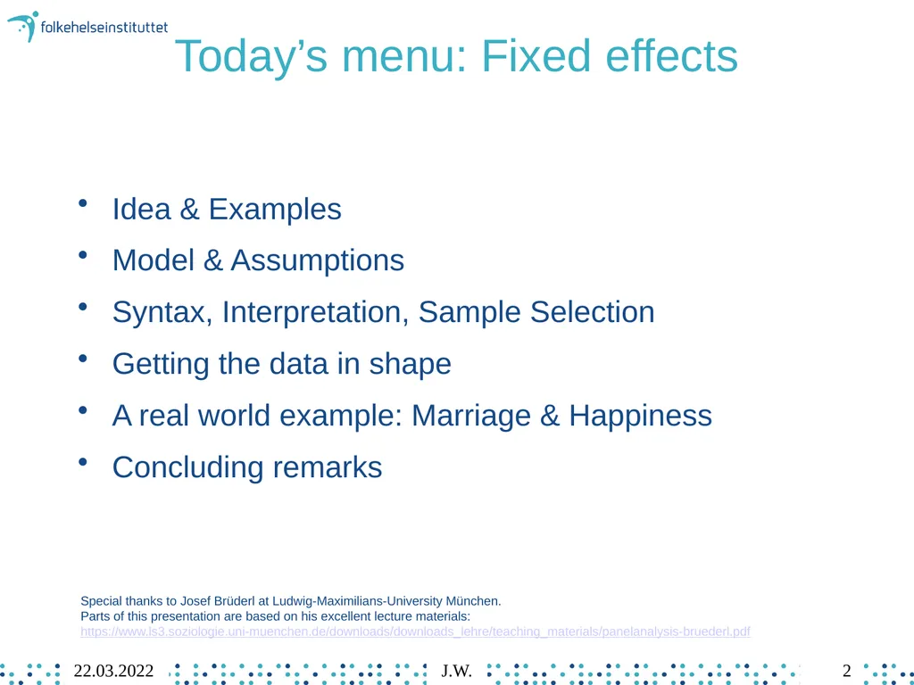
slide2. Today’s menu: Fixed effects Idea & Examples
Model & Assumptions
Syntax, Interpretation, Sample Selection
Getting the data in shape
A real world example: Marriage & Happiness
Concluding remarks Special thanks to Josef Brüderl at Ludwig-Maximilians-University München. Parts of this presentation are based on his excellent lecture materials: https://www.ls3.soziologie.uni-muenchen.de/downloads/downloads_lehre/teaching_materials/panelanalysis-bruederl.pdf 2 22.03.2022 J.W.<br>
slide3. Idea & Examples 3 22.03.2022 J.W.<br>
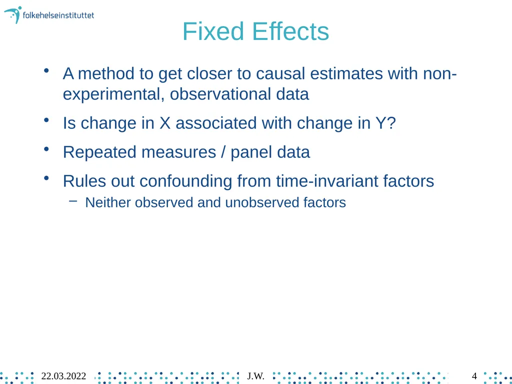
slide4. Fixed Effects A method to get closer to causal estimates with non-experimental, observational data
Is change in X associated with change in Y?
Repeated measures / panel data
Rules out confounding from time-invariant factors
Neither observed and unobserved factors 4 22.03.2022 J.W.<br>
slide5. Examples 5 22.03.2022 J.W.<br>
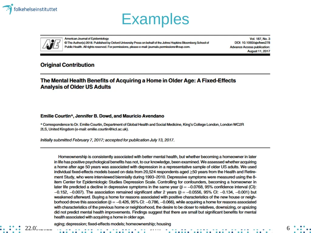
slide6. Examples 6 22.03.2022 J.W.<br>
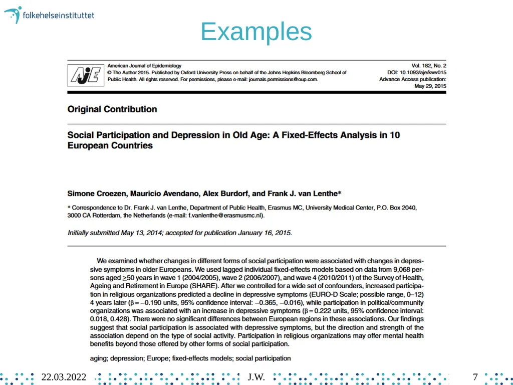
slide7. Examples 7 22.03.2022 J.W.<br>
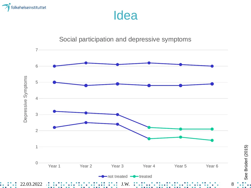
slide8. Idea See Brüderl (2015) 8 22.03.2022 J.W.<br>
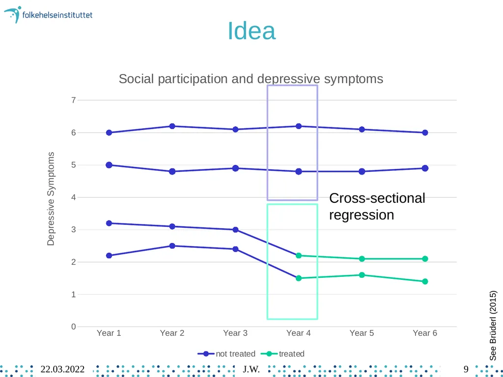
slide9. Idea Cross-sectional
regression See Brüderl (2015) 9 22.03.2022 J.W.<br>
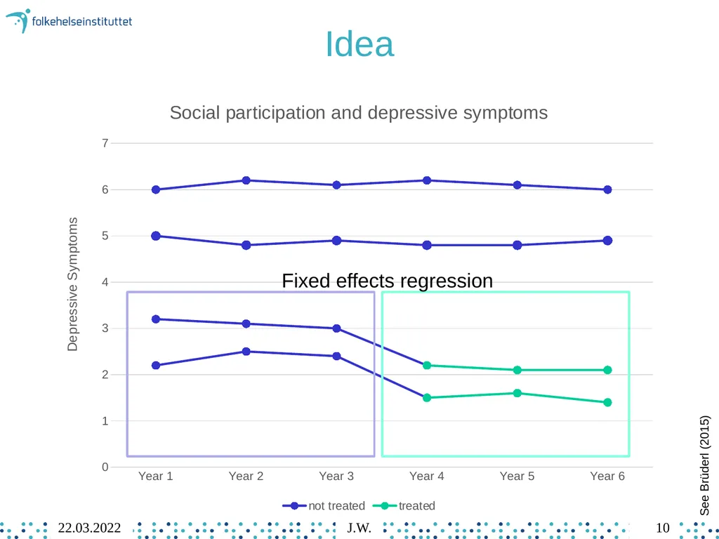
slide10. Idea Fixed effects regression See Brüderl (2015) 10 22.03.2022 J.W.<br>
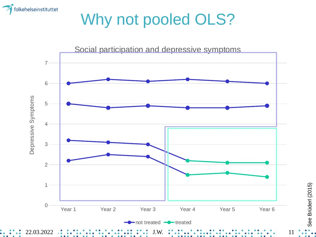
slide11. Why not pooled OLS? See Brüderl (2015) 11 22.03.2022 J.W.<br>
slide12. Model & Assumptions 12 22.03.2022 J.W.<br>
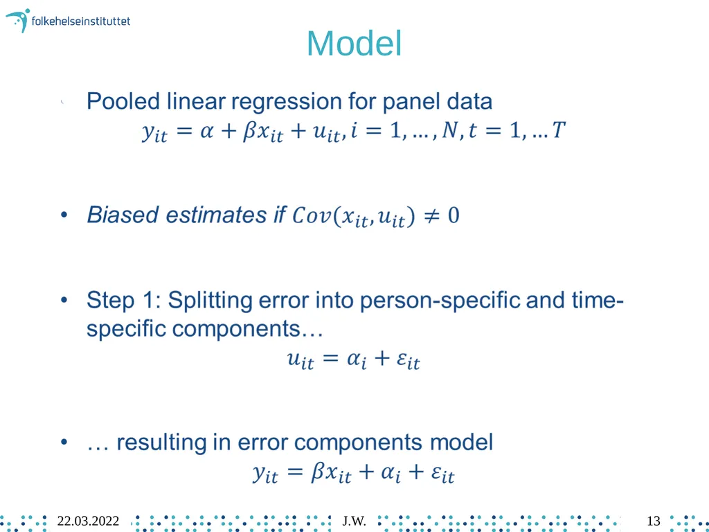
slide13. Model 13 22.03.2022 J.W.<br>
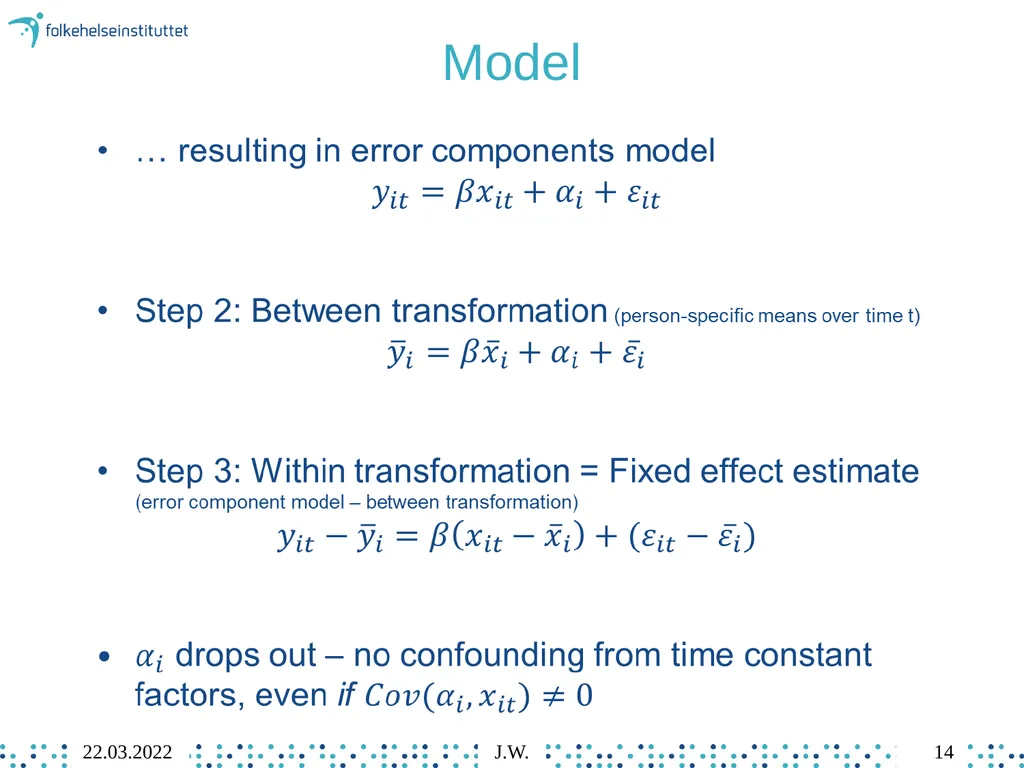
slide14. Model 14 22.03.2022 J.W.<br>
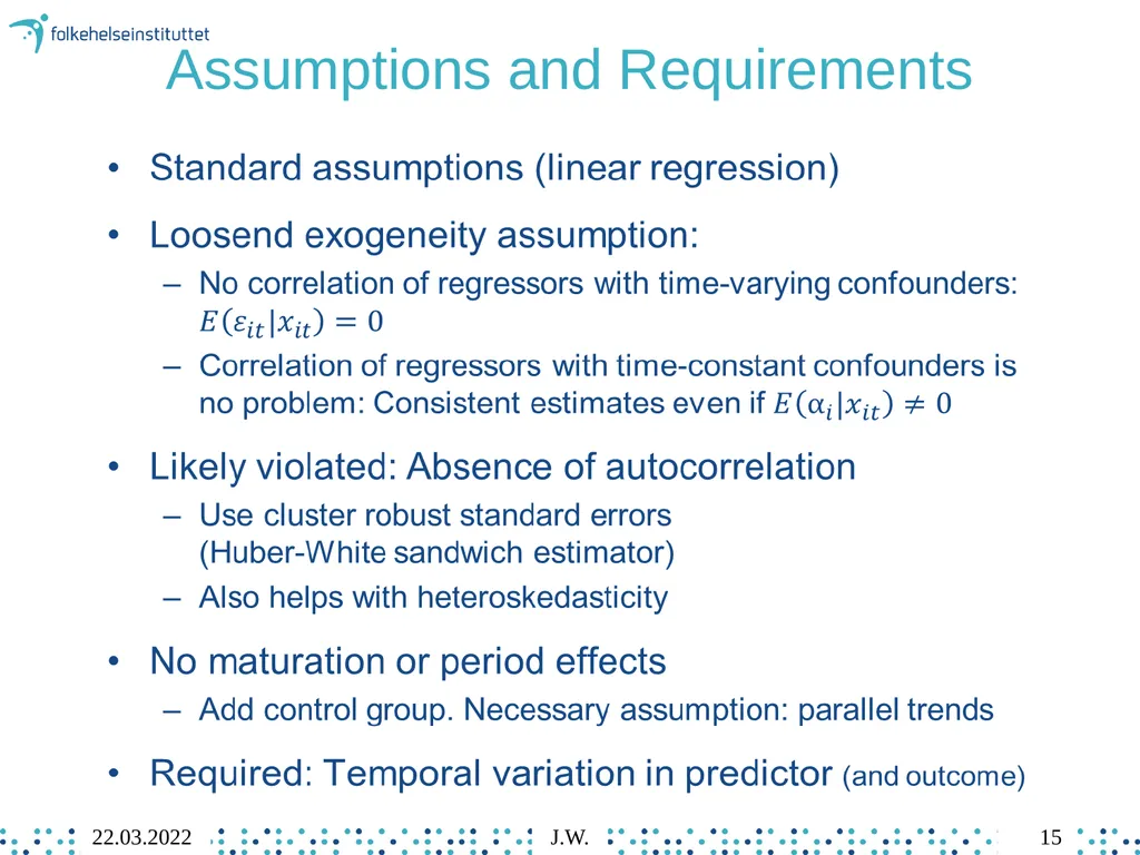
slide15. Assumptions and Requirements 15 22.03.2022 J.W.<br>
slide16. Syntax, Interpretation, Sample Selection 16 22.03.2022 J.W.<br>
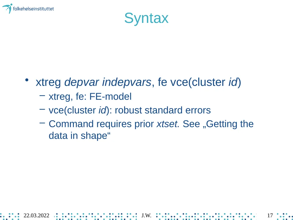
slide17. Syntax xtreg depvar indepvars, fe vce(cluster id)
xtreg, fe: FE-model
vce(cluster id): robust standard errors
Command requires prior xtset. See „Getting the data in shape“ 17 22.03.2022 J.W.<br>
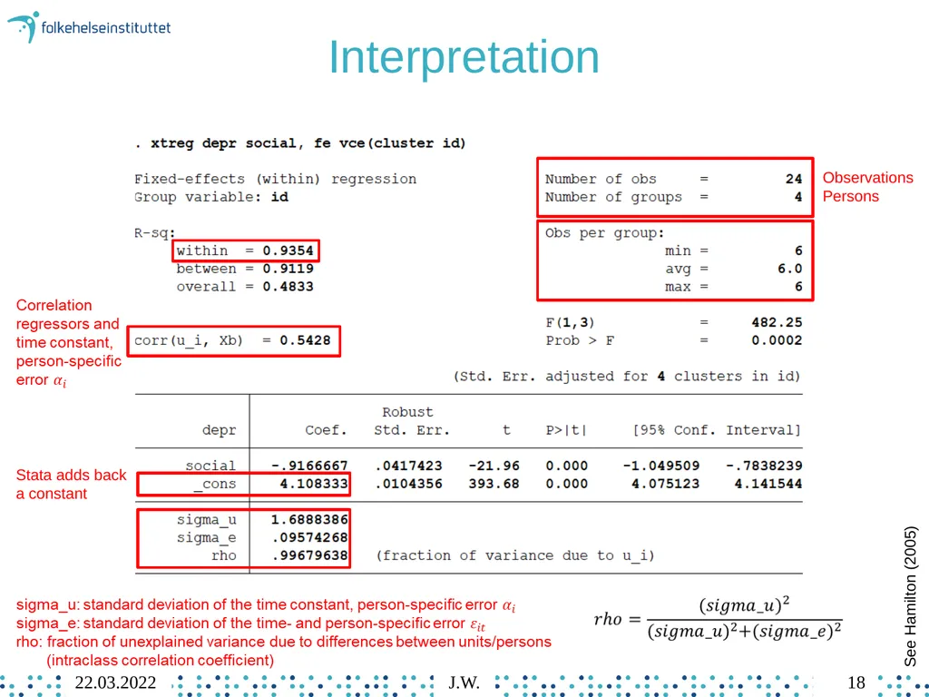
slide18. Interpretation Observations
Persons See Hamilton (2005) Stata adds back a constant 18 22.03.2022 J.W.<br>
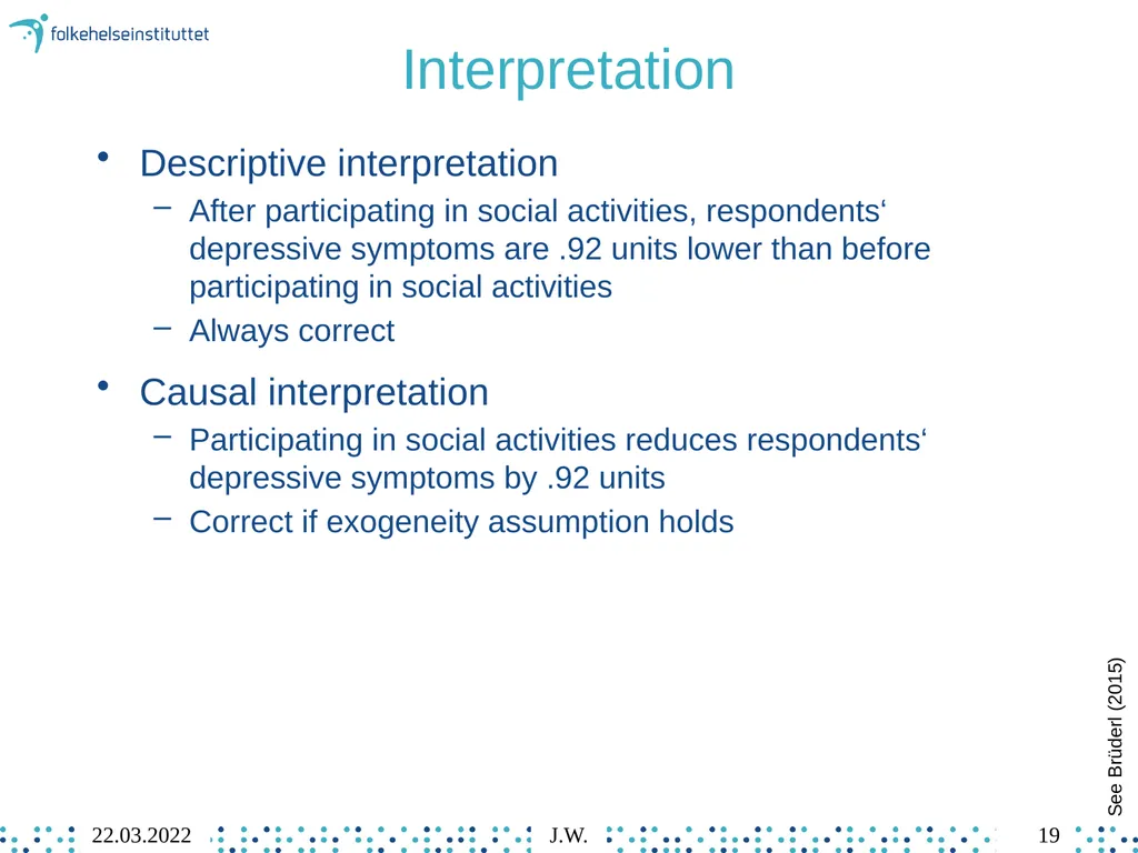
slide19. Interpretation See Brüderl (2015) Descriptive interpretation
After participating in social activities, respondents‘ depressive symptoms are .92 units lower than before participating in social activities
Always correct
Causal interpretation
Participating in social activities reduces respondents‘ depressive symptoms by .92 units
Correct if exogeneity assumption holds 19 22.03.2022 J.W.<br>
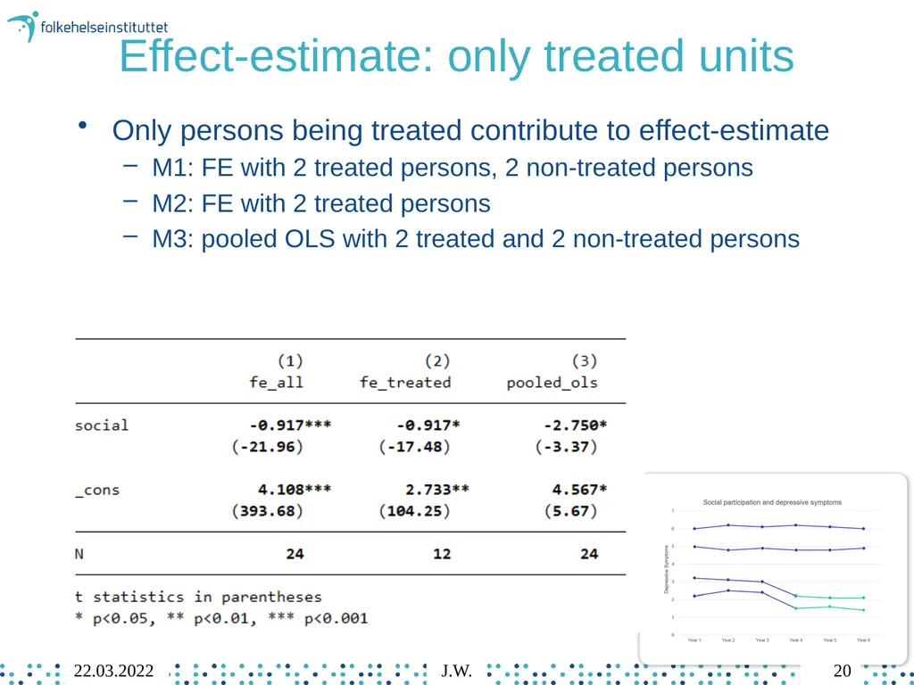
slide20. Effect-estimate: only treated units Only persons being treated contribute to effect-estimate
M1: FE with 2 treated persons, 2 non-treated persons
M2: FE with 2 treated persons
M3: pooled OLS with 2 treated and 2 non-treated persons 20 22.03.2022 J.W.<br>
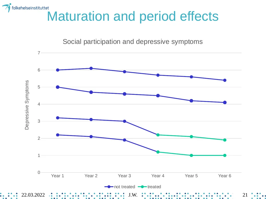
slide21. Maturation and period effects 21 22.03.2022 J.W.<br>
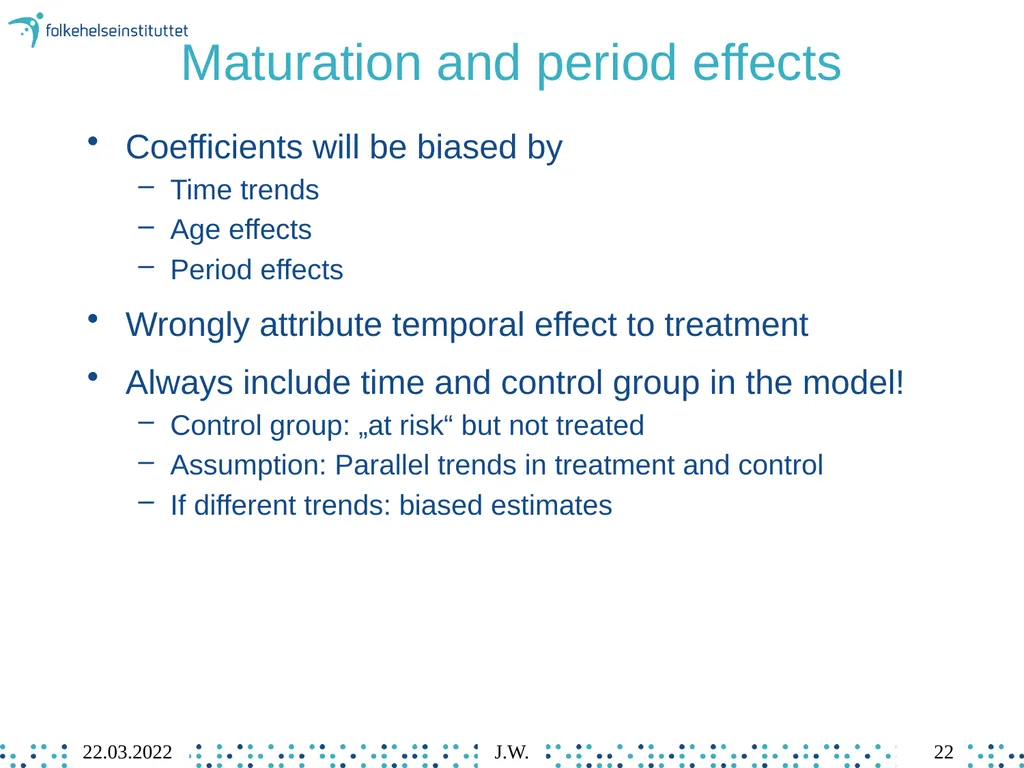
slide22. Maturation and period effects Coefficients will be biased by
Time trends
Age effects
Period effects
Wrongly attribute temporal effect to treatment
Always include time and control group in the model!
Control group: „at risk“ but not treated
Assumption: Parallel trends in treatment and control
If different trends: biased estimates 22 22.03.2022 J.W.<br>
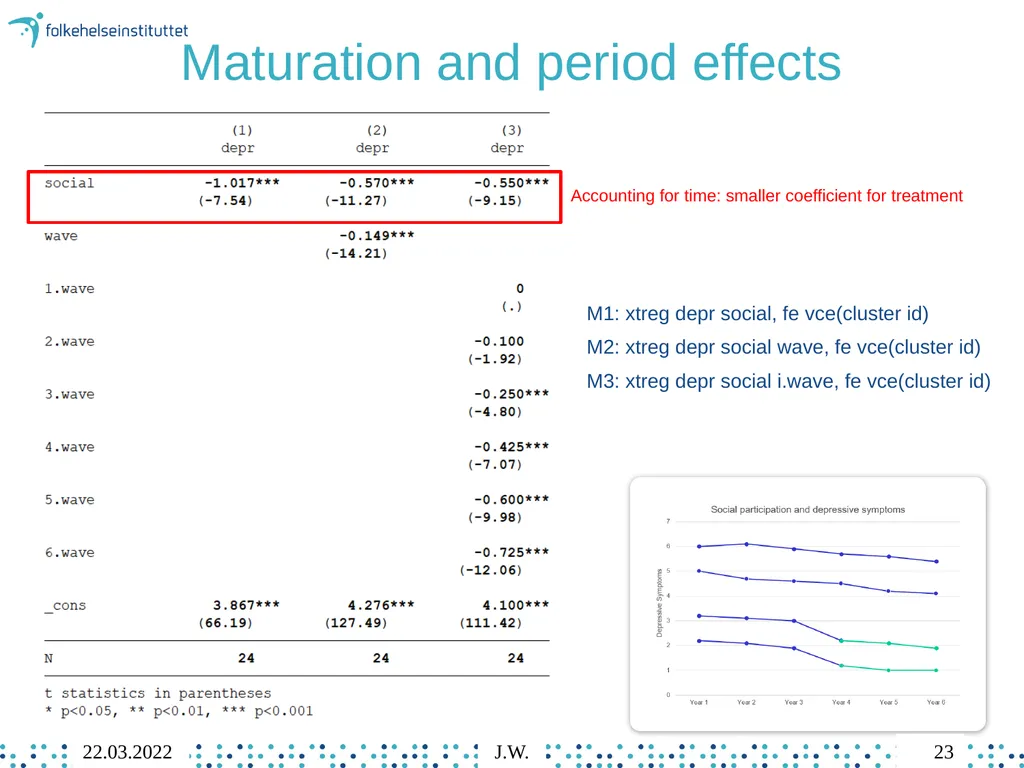
slide23. Maturation and period effects M1: xtreg depr social, fe vce(cluster id)
M2: xtreg depr social wave, fe vce(cluster id)
M3: xtreg depr social i.wave, fe vce(cluster id) Accounting for time: smaller coefficient for treatment 23 22.03.2022 J.W.<br>
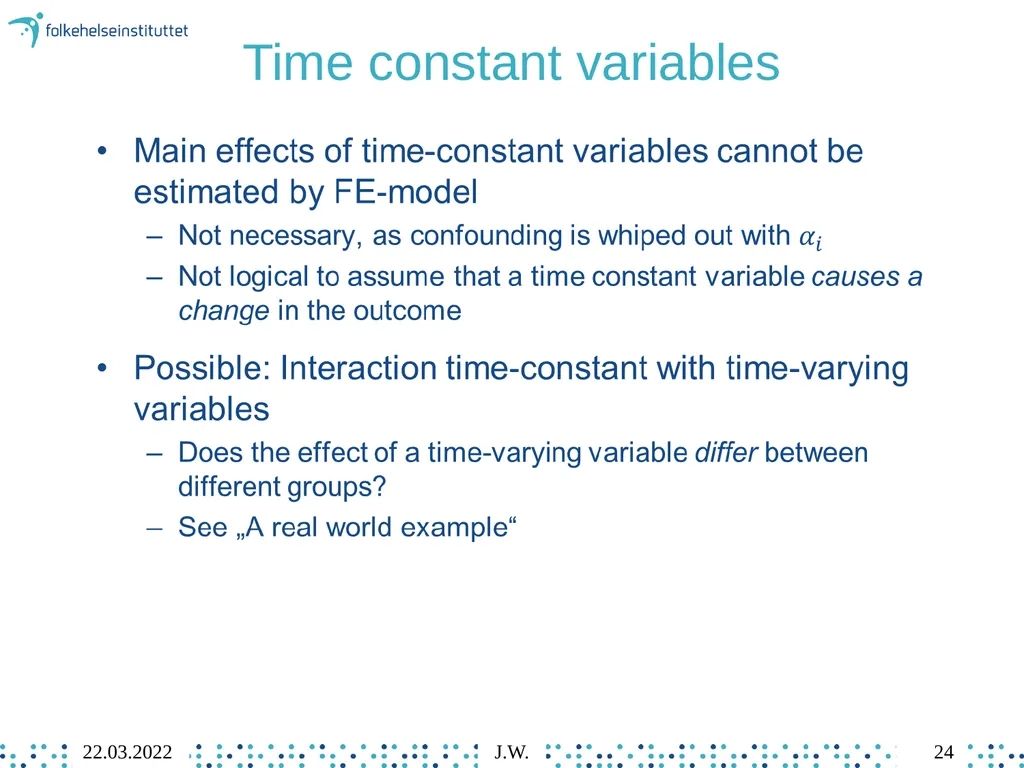
slide24. Time constant variables 24 22.03.2022 J.W.<br>
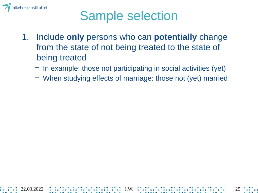
slide25. Sample selection Include only persons who can potentially change from the state of not being treated to the state of being treated
In example: those not participating in social activities (yet)
When studying effects of marriage: those not (yet) married 25 22.03.2022 J.W.<br>
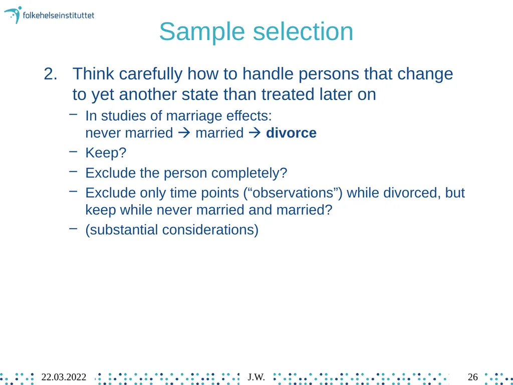
slide26. Sample selection Think carefully how to handle persons that change to yet another state than treated later on
In studies of marriage effects: never married married divorce
Keep?
Exclude the person completely?
Exclude only time points (“observations”) while divorced, but keep while never married and married?
(substantial considerations) 26 22.03.2022 J.W.<br>
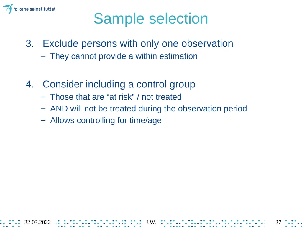
slide27. Sample selection Exclude persons with only one observation
They cannot provide a within estimation
Consider including a control group
Those that are “at risk” / not treated
AND will not be treated during the observation period
Allows controlling for time/age 27 22.03.2022 J.W.<br>
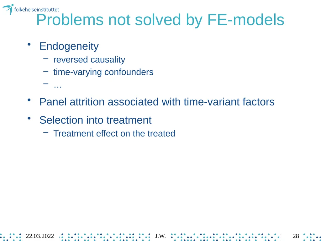
slide28. Problems not solved by FE-models Endogeneity
reversed causality
time-varying confounders
…
Panel attrition associated with time-variant factors
Selection into treatment
Treatment effect on the treated 28 22.03.2022 J.W.<br>
slide29. Getting the data in shape 29 22.03.2022 J.W.<br>
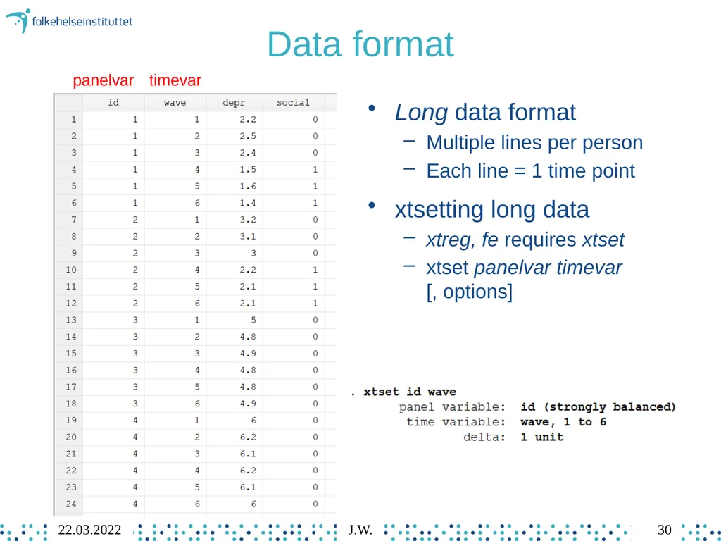
slide30. Data format Long data format
Multiple lines per person
Each line = 1 time point
xtsetting long data
xtreg, fe requires xtset
xtset panelvar timevar [, options] panelvar timevar 30 22.03.2022 J.W.<br>
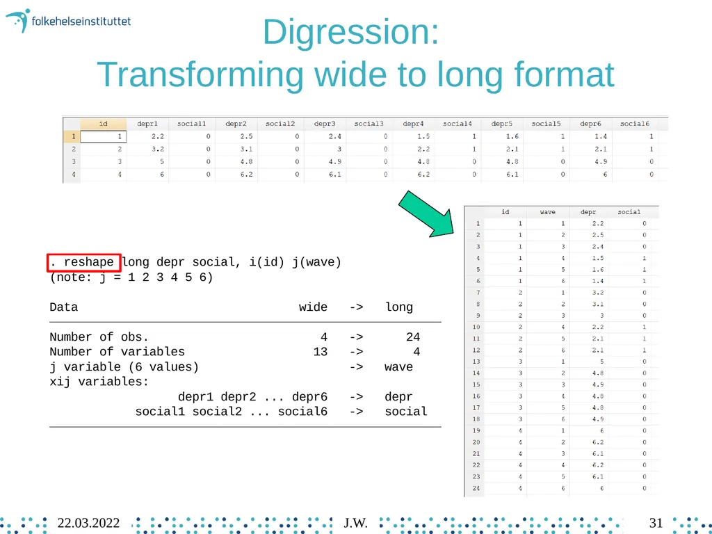
slide31. Digression: Transforming wide to long format 31 22.03.2022 J.W.<br>
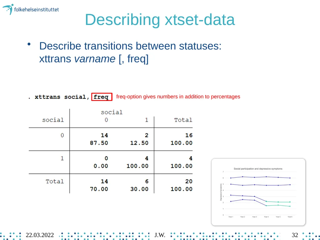
slide32. Describing xtset-data Describe transitions between statuses: xttrans varname [, freq] freq-option gives numbers in addition to percentages 32 22.03.2022 J.W.<br>
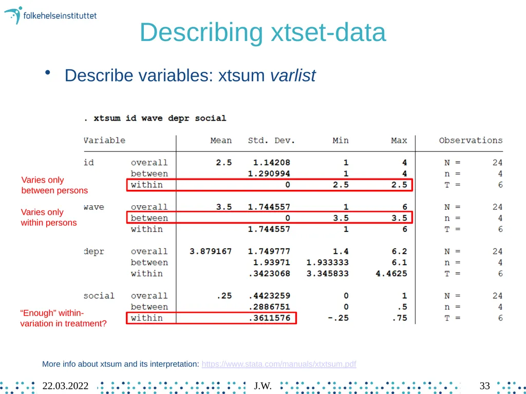
slide33. Describing xtset-data Describe variables: xtsum varlist Varies only between persons “Enough” within-
variation in treatment? Varies only within persons 33 22.03.2022 J.W. More info about xtsum and its interpretation: https://www.stata.com/manuals/xtxtsum.pdf<br>
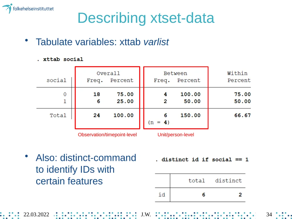
slide34. Describing xtset-data Tabulate variables: xttab varlist
Also: distinct-command to identify IDs with certain features Observation/timepoint-level Unit/person-level 34 22.03.2022 J.W.<br>
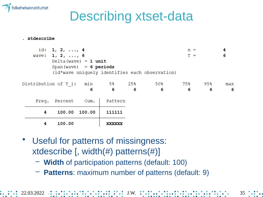
slide35. Describing xtset-data Useful for patterns of missingness: xtdescribe [, width(#) patterns(#)]
Width of participation patterns (default: 100)
Patterns: maximum number of patterns (default: 9) 35 22.03.2022 J.W.<br>
slide36. Useful commands for long data 36 J.W.<br>
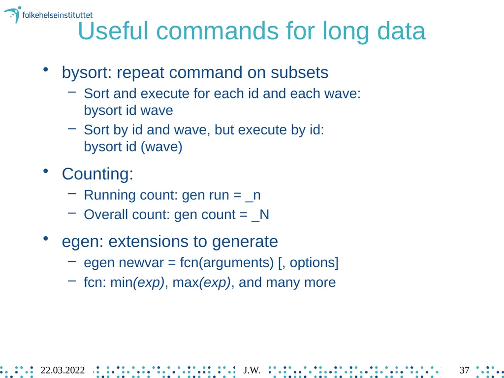
slide37. Useful commands for long data bysort: repeat command on subsets
Sort and execute for each id and each wave: bysort id wave
Sort by id and wave, but execute by id: bysort id (wave)
Counting:
Running count: gen run = _n
Overall count: gen count = _N
egen: extensions to generate
egen newvar = fcn(arguments) [, options]
fcn: min(exp), max(exp), and many more 37 22.03.2022 J.W.<br>
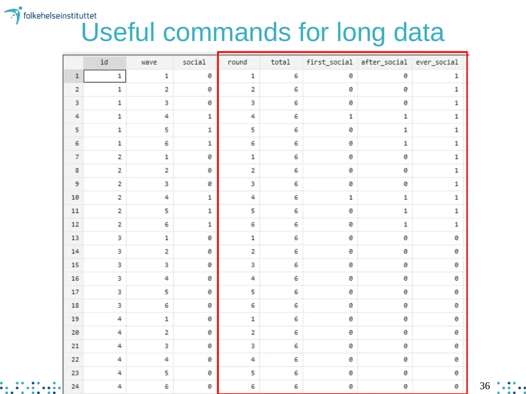
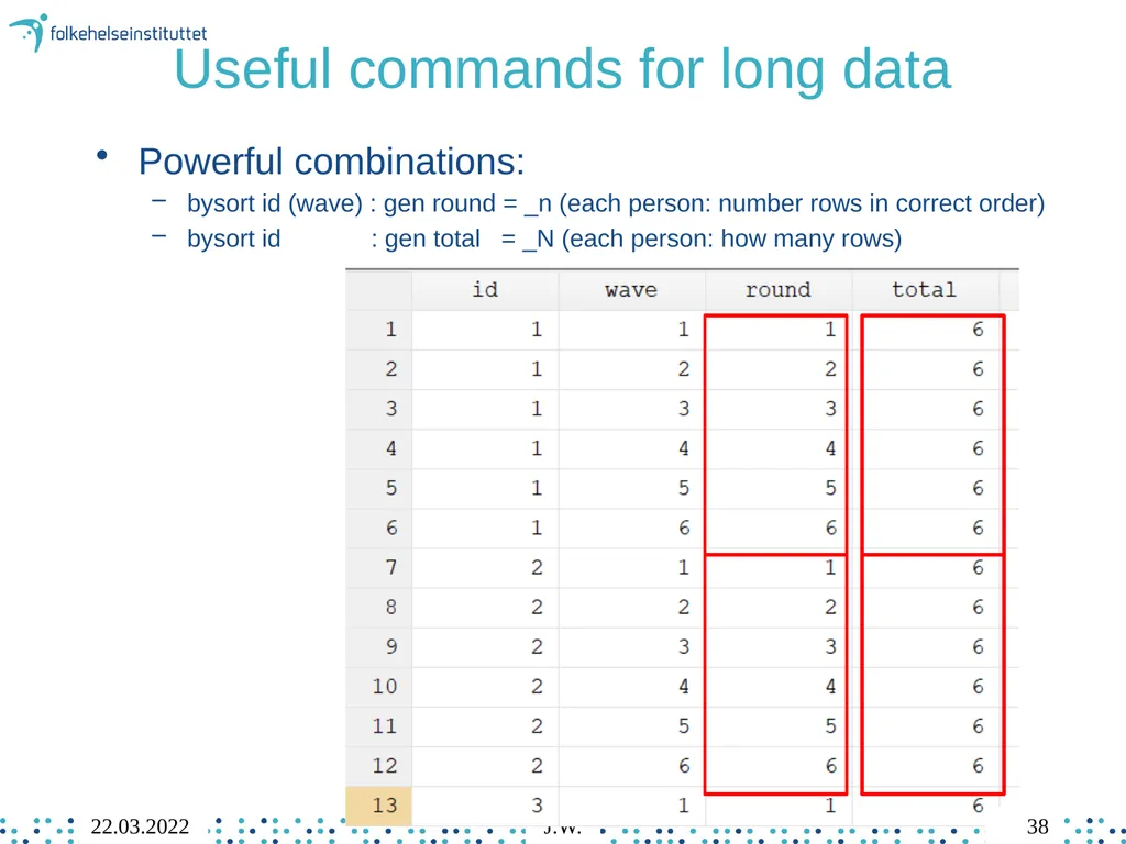
slide38. Useful commands for long data Powerful combinations:
bysort id (wave) : gen round = _n (each person: number rows in correct order)
bysort id : gen total = _N (each person: how many rows) 38 22.03.2022 J.W.<br>
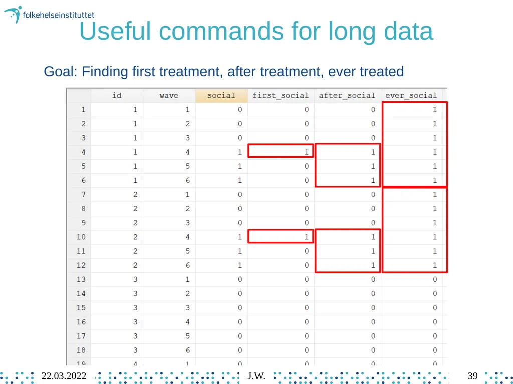
slide39. Useful commands for long data Goal: Finding first treatment, after treatment, ever treated 39 22.03.2022 J.W.<br>
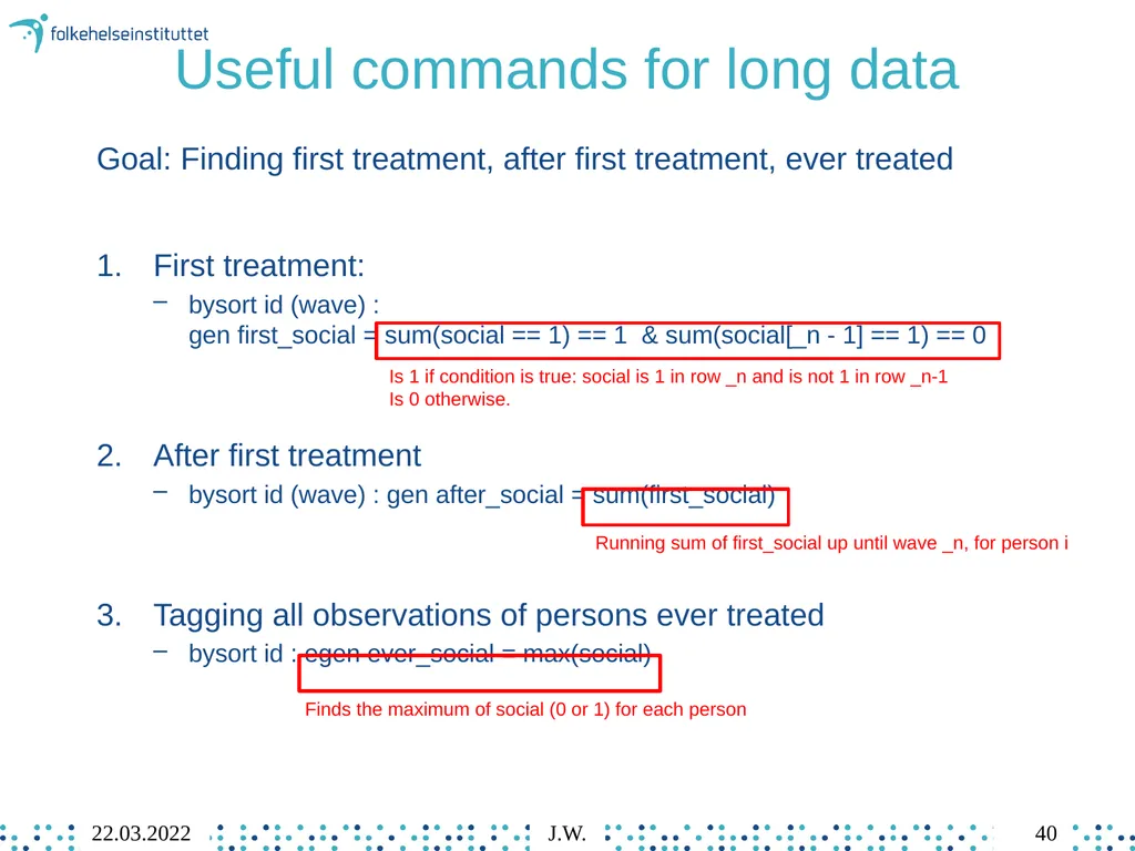
slide40. Useful commands for long data Goal: Finding first treatment, after first treatment, ever treated
First treatment:
bysort id (wave) : gen first_social = sum(social == 1) == 1 & sum(social[_n - 1] == 1) == 0
After first treatment
bysort id (wave) : gen after_social = sum(first_social)
Tagging all observations of persons ever treated
bysort id : egen ever_social = max(social) Running sum of first_social up until wave _n, for person i Finds the maximum of social (0 or 1) for each person Is 1 if condition is true: social is 1 in row _n and is not 1 in row _n-1 Is 0 otherwise. 40 22.03.2022 J.W.<br>
slide41. A real world example: Marriage & Happiness 41 22.03.2022 J.W.<br>
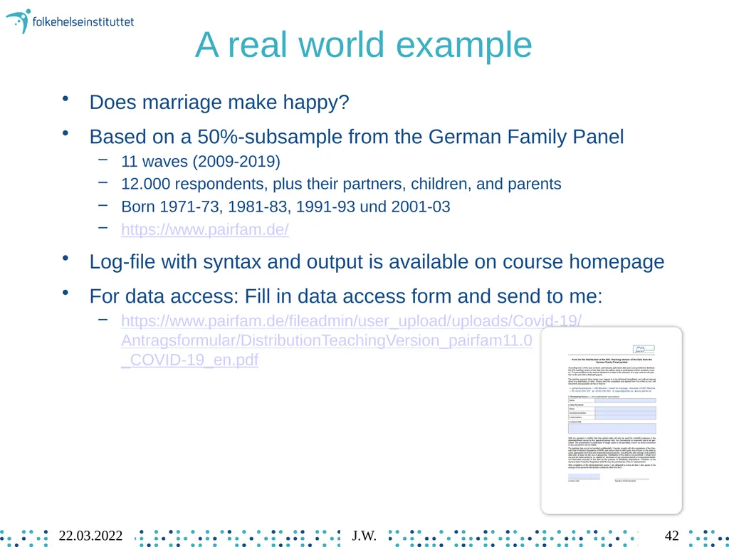
slide42. A real world example Does marriage make happy?
Based on a 50%-subsample from the German Family Panel
11 waves (2009-2019)
12.000 respondents, plus their partners, children, and parents
Born 1971-73, 1981-83, 1991-93 und 2001-03
https://www.pairfam.de/
Log-file with syntax and output is available on course homepage
For data access: Fill in data access form and send to me:
https://www.pairfam.de/fileadmin/user_upload/ uploads/Covid-19/Antragsformular/ DistributionTeachingVersion_pairfam11.0 _COVID-19_en.pdf 42 22.03.2022 J.W.<br>
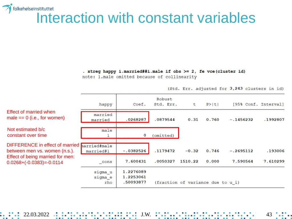
slide43. Interaction with constant variables Not estimated b/c constant over time Effect of married when male == 0 (i.e., for women) DIFFERENCE in effect of married between men vs. women (n.s.).
Effect of being married for men:
0.0268+(-0.0383)=-0.0114 43 22.03.2022 J.W.<br>
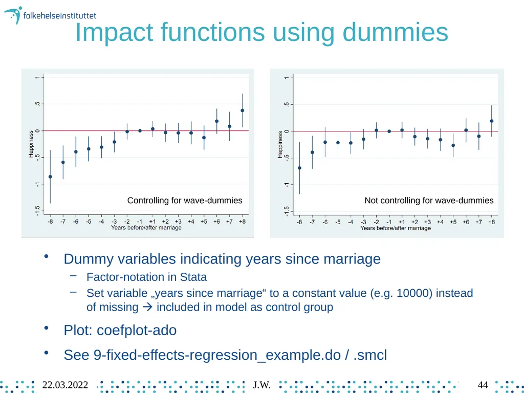
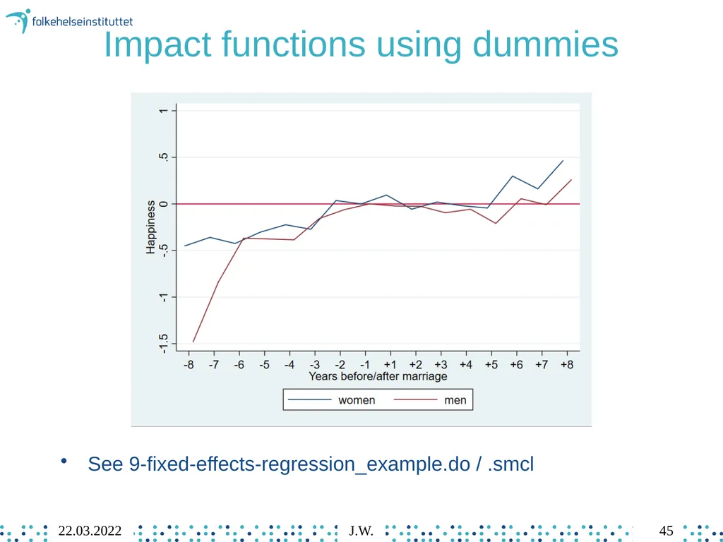
slide44. Impact functions using dummies Dummy variables indicating years since marriage
Factor-notation in Stata
Set variable „years since marriage“ to a constant value (e.g. 10000) instead of missing included in model as control group
Plot: coefplot-ado
See 9-fixed-effects-regression_example.do / .smcl Controlling for wave-dummies Not controlling for wave-dummies 44 22.03.2022 J.W.<br>
slide45. Impact functions using dummies See 9-fixed-effects-regression_example.do / .smcl 45 22.03.2022 J.W.<br>
slide46. Concluding remarks 46 22.03.2022 J.W.<br>
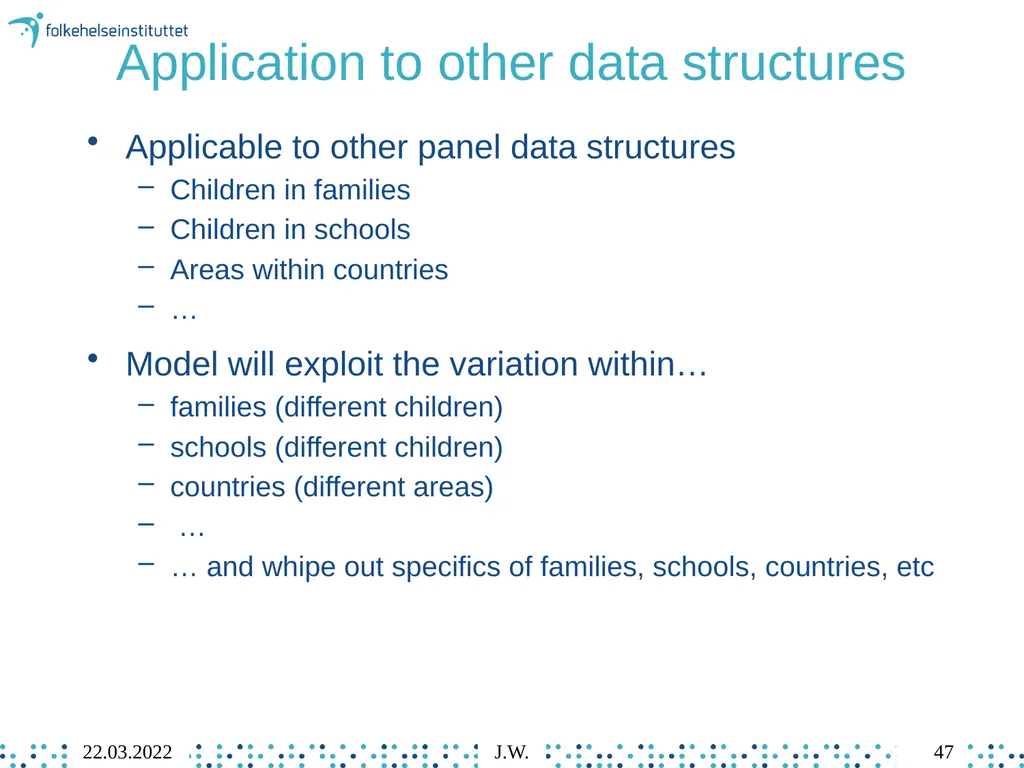
slide47. Application to other data structures Applicable to other panel data structures
Children in families
Children in schools
Areas within countries
…
Model will exploit the variation within…
families (different children)
schools (different children)
countries (different areas)
…
… and whipe out specifics of families, schools, countries, etc 47 22.03.2022 J.W.<br>
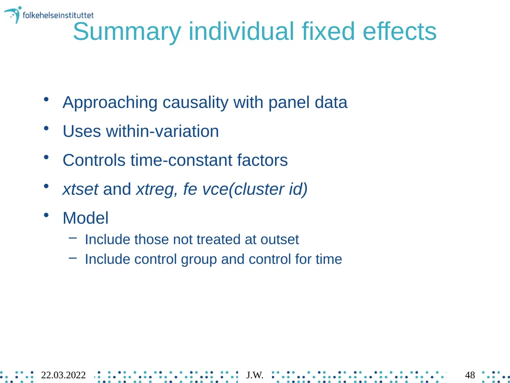
slide48. Summary individual fixed effects Approaching causality with panel data
Uses within-variation
Controls time-constant factors
xtset and xtreg, fe vce(cluster id)
Model
Include those not treated at outset
Include control group and control for time 48 22.03.2022 J.W.<br>
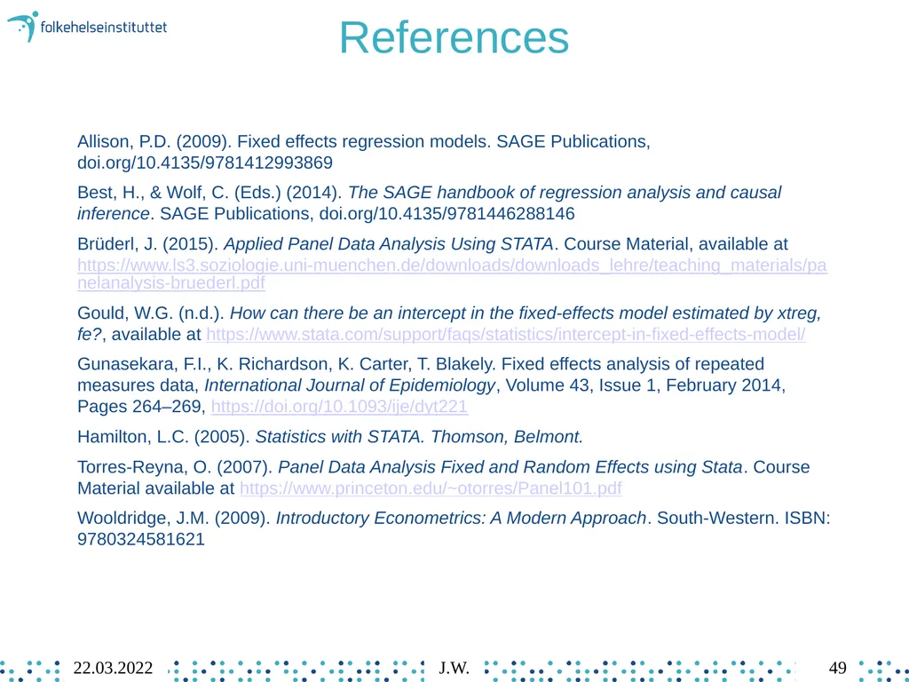
slide49. References Allison, P.D. (2009). Fixed effects regression models. SAGE Publications, doi.org/10.4135/9781412993869
Best, H., & Wolf, C. (Eds.) (2014). The SAGE handbook of regression analysis and causal inference. SAGE Publications, doi.org/10.4135/9781446288146
Brüderl, J. (2015). Applied Panel Data Analysis Using STATA. Course Material, available at https://www.ls3.soziologie.uni-muenchen.de/downloads/downloads_lehre/teaching_materials/panelanalysis-bruederl.pdf
Gould, W.G. (n.d.). How can there be an intercept in the fixed-effects model estimated by xtreg, fe?, available at https://www.stata.com/support/faqs/statistics/intercept-in-fixed-effects-model/
Gunasekara, F.I., K. Richardson, K. Carter, T. Blakely. Fixed effects analysis of repeated measures data, International Journal of Epidemiology, Volume 43, Issue 1, February 2014, Pages 264–269, https://doi.org/10.1093/ije/dyt221
Hamilton, L.C. (2005). Statistics with STATA. Thomson, Belmont.
Torres-Reyna, O. (2007). Panel Data Analysis Fixed and Random Effects using Stata. Course Material available at https://www.princeton.edu/~otorres/Panel101.pdf
Wooldridge, J.M. (2009). Introductory Econometrics: A Modern Approach. South-Western. ISBN: 9780324581621 49 22.03.2022 J.W.<br>
Presentation, data and programs at:
https://bit.ly/3ItnOGj 1 22.03.2022 J.W.<br>
slide2. Today’s menu: Fixed effects Idea & Examples
Model & Assumptions
Syntax, Interpretation, Sample Selection
Getting the data in shape
A real world example: Marriage & Happiness
Concluding remarks Special thanks to Josef Brüderl at Ludwig-Maximilians-University München. Parts of this presentation are based on his excellent lecture materials: https://www.ls3.soziologie.uni-muenchen.de/downloads/downloads_lehre/teaching_materials/panelanalysis-bruederl.pdf 2 22.03.2022 J.W.<br>
slide3. Idea & Examples 3 22.03.2022 J.W.<br>
slide4. Fixed Effects A method to get closer to causal estimates with non-experimental, observational data
Is change in X associated with change in Y?
Repeated measures / panel data
Rules out confounding from time-invariant factors
Neither observed and unobserved factors 4 22.03.2022 J.W.<br>
slide5. Examples 5 22.03.2022 J.W.<br>
slide6. Examples 6 22.03.2022 J.W.<br>
slide7. Examples 7 22.03.2022 J.W.<br>
slide8. Idea See Brüderl (2015) 8 22.03.2022 J.W.<br>
slide9. Idea Cross-sectional
regression See Brüderl (2015) 9 22.03.2022 J.W.<br>
slide10. Idea Fixed effects regression See Brüderl (2015) 10 22.03.2022 J.W.<br>
slide11. Why not pooled OLS? See Brüderl (2015) 11 22.03.2022 J.W.<br>
slide12. Model & Assumptions 12 22.03.2022 J.W.<br>
slide13. Model 13 22.03.2022 J.W.<br>
slide14. Model 14 22.03.2022 J.W.<br>
slide15. Assumptions and Requirements 15 22.03.2022 J.W.<br>
slide16. Syntax, Interpretation, Sample Selection 16 22.03.2022 J.W.<br>
slide17. Syntax xtreg depvar indepvars, fe vce(cluster id)
xtreg, fe: FE-model
vce(cluster id): robust standard errors
Command requires prior xtset. See „Getting the data in shape“ 17 22.03.2022 J.W.<br>
slide18. Interpretation Observations
Persons See Hamilton (2005) Stata adds back a constant 18 22.03.2022 J.W.<br>
slide19. Interpretation See Brüderl (2015) Descriptive interpretation
After participating in social activities, respondents‘ depressive symptoms are .92 units lower than before participating in social activities
Always correct
Causal interpretation
Participating in social activities reduces respondents‘ depressive symptoms by .92 units
Correct if exogeneity assumption holds 19 22.03.2022 J.W.<br>
slide20. Effect-estimate: only treated units Only persons being treated contribute to effect-estimate
M1: FE with 2 treated persons, 2 non-treated persons
M2: FE with 2 treated persons
M3: pooled OLS with 2 treated and 2 non-treated persons 20 22.03.2022 J.W.<br>
slide21. Maturation and period effects 21 22.03.2022 J.W.<br>
slide22. Maturation and period effects Coefficients will be biased by
Time trends
Age effects
Period effects
Wrongly attribute temporal effect to treatment
Always include time and control group in the model!
Control group: „at risk“ but not treated
Assumption: Parallel trends in treatment and control
If different trends: biased estimates 22 22.03.2022 J.W.<br>
slide23. Maturation and period effects M1: xtreg depr social, fe vce(cluster id)
M2: xtreg depr social wave, fe vce(cluster id)
M3: xtreg depr social i.wave, fe vce(cluster id) Accounting for time: smaller coefficient for treatment 23 22.03.2022 J.W.<br>
slide24. Time constant variables 24 22.03.2022 J.W.<br>
slide25. Sample selection Include only persons who can potentially change from the state of not being treated to the state of being treated
In example: those not participating in social activities (yet)
When studying effects of marriage: those not (yet) married 25 22.03.2022 J.W.<br>
slide26. Sample selection Think carefully how to handle persons that change to yet another state than treated later on
In studies of marriage effects: never married married divorce
Keep?
Exclude the person completely?
Exclude only time points (“observations”) while divorced, but keep while never married and married?
(substantial considerations) 26 22.03.2022 J.W.<br>
slide27. Sample selection Exclude persons with only one observation
They cannot provide a within estimation
Consider including a control group
Those that are “at risk” / not treated
AND will not be treated during the observation period
Allows controlling for time/age 27 22.03.2022 J.W.<br>
slide28. Problems not solved by FE-models Endogeneity
reversed causality
time-varying confounders
…
Panel attrition associated with time-variant factors
Selection into treatment
Treatment effect on the treated 28 22.03.2022 J.W.<br>
slide29. Getting the data in shape 29 22.03.2022 J.W.<br>
slide30. Data format Long data format
Multiple lines per person
Each line = 1 time point
xtsetting long data
xtreg, fe requires xtset
xtset panelvar timevar [, options] panelvar timevar 30 22.03.2022 J.W.<br>
slide31. Digression: Transforming wide to long format 31 22.03.2022 J.W.<br>
slide32. Describing xtset-data Describe transitions between statuses: xttrans varname [, freq] freq-option gives numbers in addition to percentages 32 22.03.2022 J.W.<br>
slide33. Describing xtset-data Describe variables: xtsum varlist Varies only between persons “Enough” within-
variation in treatment? Varies only within persons 33 22.03.2022 J.W. More info about xtsum and its interpretation: https://www.stata.com/manuals/xtxtsum.pdf<br>
slide34. Describing xtset-data Tabulate variables: xttab varlist
Also: distinct-command to identify IDs with certain features Observation/timepoint-level Unit/person-level 34 22.03.2022 J.W.<br>
slide35. Describing xtset-data Useful for patterns of missingness: xtdescribe [, width(#) patterns(#)]
Width of participation patterns (default: 100)
Patterns: maximum number of patterns (default: 9) 35 22.03.2022 J.W.<br>
slide36. Useful commands for long data 36 J.W.<br>
slide37. Useful commands for long data bysort: repeat command on subsets
Sort and execute for each id and each wave: bysort id wave
Sort by id and wave, but execute by id: bysort id (wave)
Counting:
Running count: gen run = _n
Overall count: gen count = _N
egen: extensions to generate
egen newvar = fcn(arguments) [, options]
fcn: min(exp), max(exp), and many more 37 22.03.2022 J.W.<br>
slide38. Useful commands for long data Powerful combinations:
bysort id (wave) : gen round = _n (each person: number rows in correct order)
bysort id : gen total = _N (each person: how many rows) 38 22.03.2022 J.W.<br>
slide39. Useful commands for long data Goal: Finding first treatment, after treatment, ever treated 39 22.03.2022 J.W.<br>
slide40. Useful commands for long data Goal: Finding first treatment, after first treatment, ever treated
First treatment:
bysort id (wave) : gen first_social = sum(social == 1) == 1 & sum(social[_n - 1] == 1) == 0
After first treatment
bysort id (wave) : gen after_social = sum(first_social)
Tagging all observations of persons ever treated
bysort id : egen ever_social = max(social) Running sum of first_social up until wave _n, for person i Finds the maximum of social (0 or 1) for each person Is 1 if condition is true: social is 1 in row _n and is not 1 in row _n-1 Is 0 otherwise. 40 22.03.2022 J.W.<br>
slide41. A real world example: Marriage & Happiness 41 22.03.2022 J.W.<br>
slide42. A real world example Does marriage make happy?
Based on a 50%-subsample from the German Family Panel
11 waves (2009-2019)
12.000 respondents, plus their partners, children, and parents
Born 1971-73, 1981-83, 1991-93 und 2001-03
https://www.pairfam.de/
Log-file with syntax and output is available on course homepage
For data access: Fill in data access form and send to me:
https://www.pairfam.de/fileadmin/user_upload/ uploads/Covid-19/Antragsformular/ DistributionTeachingVersion_pairfam11.0 _COVID-19_en.pdf 42 22.03.2022 J.W.<br>
slide43. Interaction with constant variables Not estimated b/c constant over time Effect of married when male == 0 (i.e., for women) DIFFERENCE in effect of married between men vs. women (n.s.).
Effect of being married for men:
0.0268+(-0.0383)=-0.0114 43 22.03.2022 J.W.<br>
slide44. Impact functions using dummies Dummy variables indicating years since marriage
Factor-notation in Stata
Set variable „years since marriage“ to a constant value (e.g. 10000) instead of missing included in model as control group
Plot: coefplot-ado
See 9-fixed-effects-regression_example.do / .smcl Controlling for wave-dummies Not controlling for wave-dummies 44 22.03.2022 J.W.<br>
slide45. Impact functions using dummies See 9-fixed-effects-regression_example.do / .smcl 45 22.03.2022 J.W.<br>
slide46. Concluding remarks 46 22.03.2022 J.W.<br>
slide47. Application to other data structures Applicable to other panel data structures
Children in families
Children in schools
Areas within countries
…
Model will exploit the variation within…
families (different children)
schools (different children)
countries (different areas)
…
… and whipe out specifics of families, schools, countries, etc 47 22.03.2022 J.W.<br>
slide48. Summary individual fixed effects Approaching causality with panel data
Uses within-variation
Controls time-constant factors
xtset and xtreg, fe vce(cluster id)
Model
Include those not treated at outset
Include control group and control for time 48 22.03.2022 J.W.<br>
slide49. References Allison, P.D. (2009). Fixed effects regression models. SAGE Publications, doi.org/10.4135/9781412993869
Best, H., & Wolf, C. (Eds.) (2014). The SAGE handbook of regression analysis and causal inference. SAGE Publications, doi.org/10.4135/9781446288146
Brüderl, J. (2015). Applied Panel Data Analysis Using STATA. Course Material, available at https://www.ls3.soziologie.uni-muenchen.de/downloads/downloads_lehre/teaching_materials/panelanalysis-bruederl.pdf
Gould, W.G. (n.d.). How can there be an intercept in the fixed-effects model estimated by xtreg, fe?, available at https://www.stata.com/support/faqs/statistics/intercept-in-fixed-effects-model/
Gunasekara, F.I., K. Richardson, K. Carter, T. Blakely. Fixed effects analysis of repeated measures data, International Journal of Epidemiology, Volume 43, Issue 1, February 2014, Pages 264–269, https://doi.org/10.1093/ije/dyt221
Hamilton, L.C. (2005). Statistics with STATA. Thomson, Belmont.
Torres-Reyna, O. (2007). Panel Data Analysis Fixed and Random Effects using Stata. Course Material available at https://www.princeton.edu/~otorres/Panel101.pdf
Wooldridge, J.M. (2009). Introductory Econometrics: A Modern Approach. South-Western. ISBN: 9780324581621 49 22.03.2022 J.W.<br>