
Adapted from notes by Prof. Stuart A. Long 1 Notes
PC
Published · 41 slides · 0 views
1 / 1
Description
Adapted from notes by Prof. Stuart A. Long 1 Notes 4 Maxwells Equations ECE 3317 Applied Electromagnetic Waves Prof. David R. Jackson Fall 2025 2 Here we present an overview of Maxwells equations. A much more thorough discussion of
Related Topics
Share
Embed code
Download this presentation From Below
"Adapted from notes by Prof. Stuart A. Long 1 Notes" is the property of its rightful owner. Permission is granted to download and print the materials on this website for personal, non-commercial use only, and to display it on your personal computer provided you do not modify the materials and that you retain all copyright notices contained in the materials. By downloading content from our website, you accept the terms of this agreement.
Presentation Transcript
01
Adapted from notes by Prof. Stuart A. Long 1 Notes 4
Maxwell’s Equations ECE 3317
Applied Electromagnetic Waves
Prof. David R. Jackson
Fall 2025<br>
Applied Electromagnetic Waves
Prof. David R. Jackson
Fall 2025<br>
02
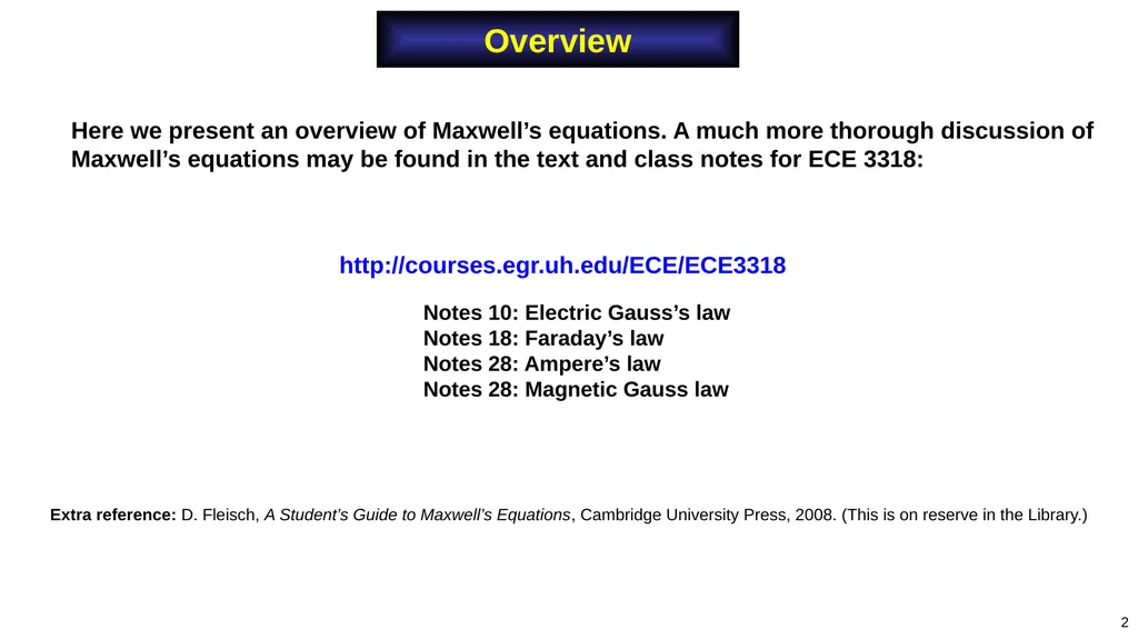
2 Here we present an overview of Maxwell’s equations. A much more thorough discussion of Maxwell’s equations may be found in the text and class notes for ECE 3318: http://courses.egr.uh.edu/ECE/ECE3318 Notes 10: Electric Gauss’s law
Notes 18: Faraday’s law
Notes 28: Ampere’s law
Notes 28: Magnetic Gauss law Extra reference: D. Fleisch, A Student’s Guide to Maxwell’s Equations, Cambridge University Press, 2008. (This is on reserve in the Library.) Overview<br>
Notes 18: Faraday’s law
Notes 28: Ampere’s law
Notes 28: Magnetic Gauss law Extra reference: D. Fleisch, A Student’s Guide to Maxwell’s Equations, Cambridge University Press, 2008. (This is on reserve in the Library.) Overview<br>
03
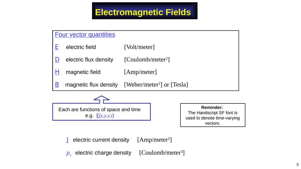
Electromagnetic Fields Four vector quantities
E electric field [Volt/meter]
D electric flux density [Coulomb/meter2]
H magnetic field [Amp/meter]
B magnetic flux density [Weber/meter2] or [Tesla] Each are functions of space and time
e.g. E(x,y,z,t) J electric current density [Amp/meter2]
ρv electric charge density [Coulomb/meter3] 3 Reminder:
The Handscript SF font is used to denote time-varying vectors.<br>
E electric field [Volt/meter]
D electric flux density [Coulomb/meter2]
H magnetic field [Amp/meter]
B magnetic flux density [Weber/meter2] or [Tesla] Each are functions of space and time
e.g. E(x,y,z,t) J electric current density [Amp/meter2]
ρv electric charge density [Coulomb/meter3] 3 Reminder:
The Handscript SF font is used to denote time-varying vectors.<br>
04
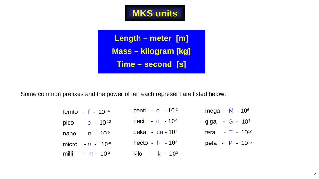
MKS units Length – meter [m]
Mass – kilogram [kg]
Time – second [s] femto - f - 10-15
pico - p - 10-12
nano - n - 10-9
micro - μ - 10-6
milli - m - 10-3 mega - M - 106
giga - G - 109
tera - T - 1012
peta - P - 1015 centi - c - 10-2
deci - d - 10-1
deka - da - 101
hecto - h - 102
kilo - k - 103 4 Some common prefixes and the power of ten each represent are listed below:<br>
Mass – kilogram [kg]
Time – second [s] femto - f - 10-15
pico - p - 10-12
nano - n - 10-9
micro - μ - 10-6
milli - m - 10-3 mega - M - 106
giga - G - 109
tera - T - 1012
peta - P - 1015 centi - c - 10-2
deci - d - 10-1
deka - da - 101
hecto - h - 102
kilo - k - 103 4 Some common prefixes and the power of ten each represent are listed below:<br>
05
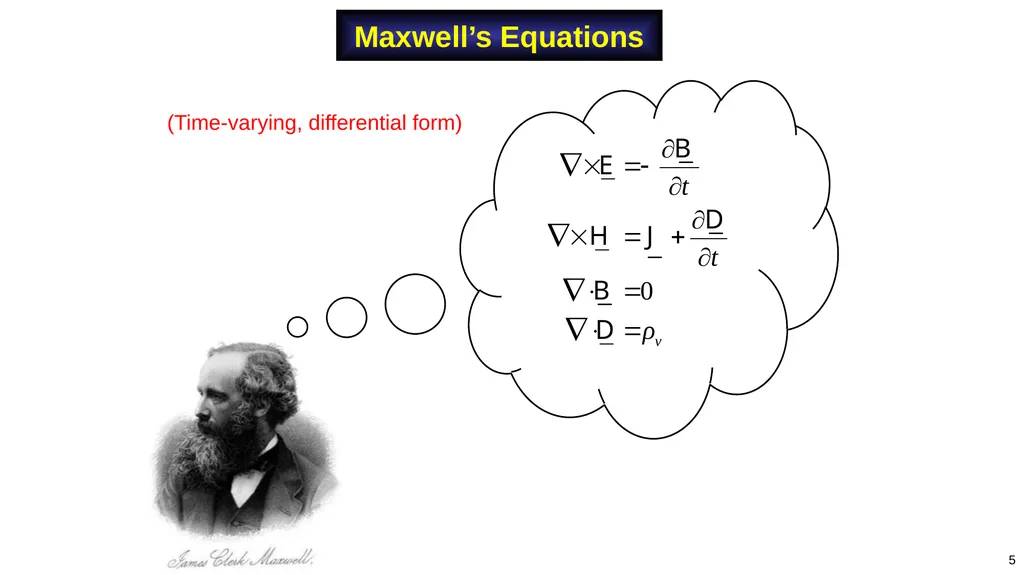
Maxwell’s Equations (Time-varying, differential form) 5<br>
06
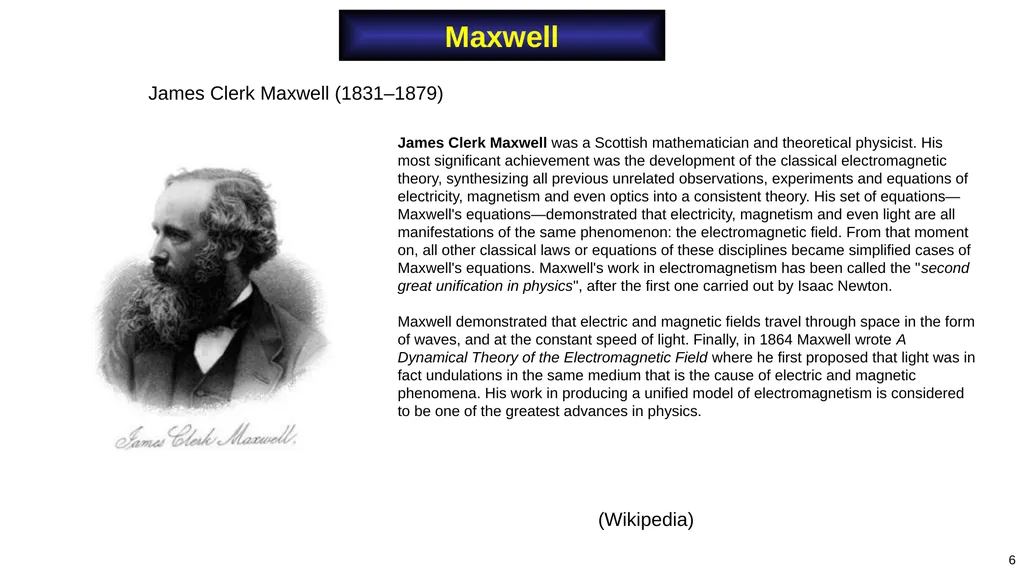
Maxwell James Clerk Maxwell (1831–1879) James Clerk Maxwell was a Scottish mathematician and theoretical physicist. His most significant achievement was the development of the classical electromagnetic theory, synthesizing all previous unrelated observations, experiments and equations of electricity, magnetism and even optics into a consistent theory. His set of equations—Maxwell's equations—demonstrated that electricity, magnetism and even light are all manifestations of the same phenomenon: the electromagnetic field. From that moment on, all other classical laws or equations of these disciplines became simplified cases of Maxwell's equations. Maxwell's work in electromagnetism has been called the "second great unification in physics", after the first one carried out by Isaac Newton.
Maxwell demonstrated that electric and magnetic fields travel through space in the form of waves, and at the constant speed of light. Finally, in 1864 Maxwell wrote A Dynamical Theory of the Electromagnetic Field where he first proposed that light was in fact undulations in the same medium that is the cause of electric and magnetic phenomena. His work in producing a unified model of electromagnetism is considered to be one of the greatest advances in physics. (Wikipedia) 6<br>
Maxwell demonstrated that electric and magnetic fields travel through space in the form of waves, and at the constant speed of light. Finally, in 1864 Maxwell wrote A Dynamical Theory of the Electromagnetic Field where he first proposed that light was in fact undulations in the same medium that is the cause of electric and magnetic phenomena. His work in producing a unified model of electromagnetism is considered to be one of the greatest advances in physics. (Wikipedia) 6<br>
07
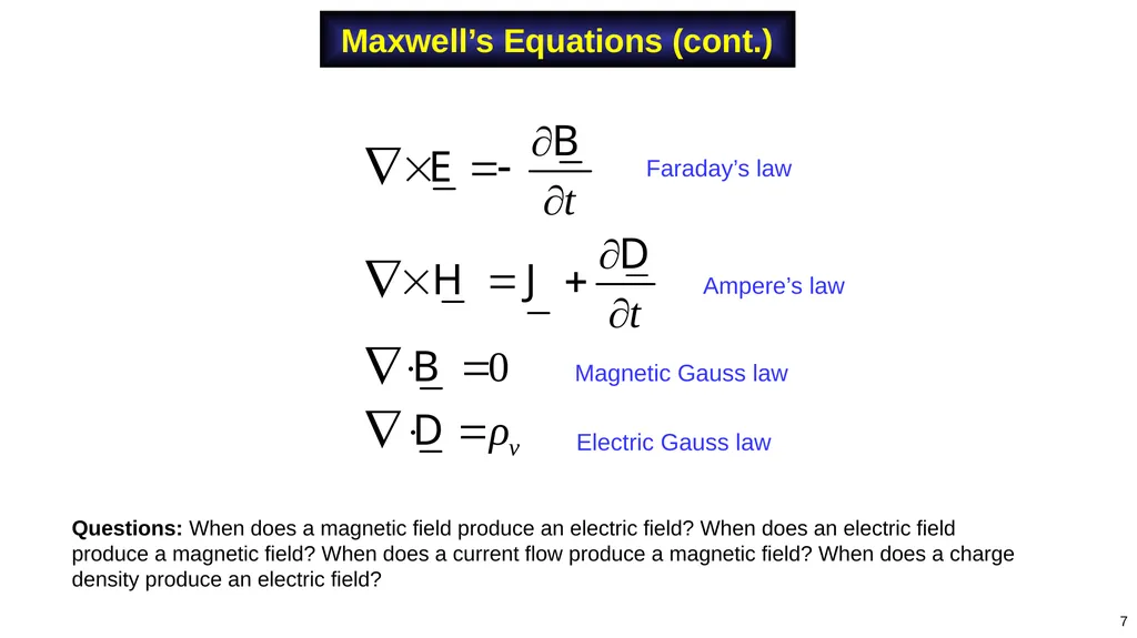
Maxwell’s Equations (cont.) Faraday’s law Ampere’s law Magnetic Gauss law Electric Gauss law 7 Questions: When does a magnetic field produce an electric field? When does an electric field produce a magnetic field? When does a current flow produce a magnetic field? When does a charge density produce an electric field?<br>
08
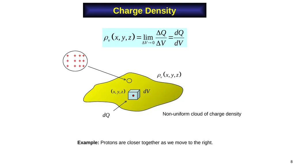
Charge Density 8 Example: Protons are closer together as we move to the right. Non-uniform cloud of charge density<br>
09
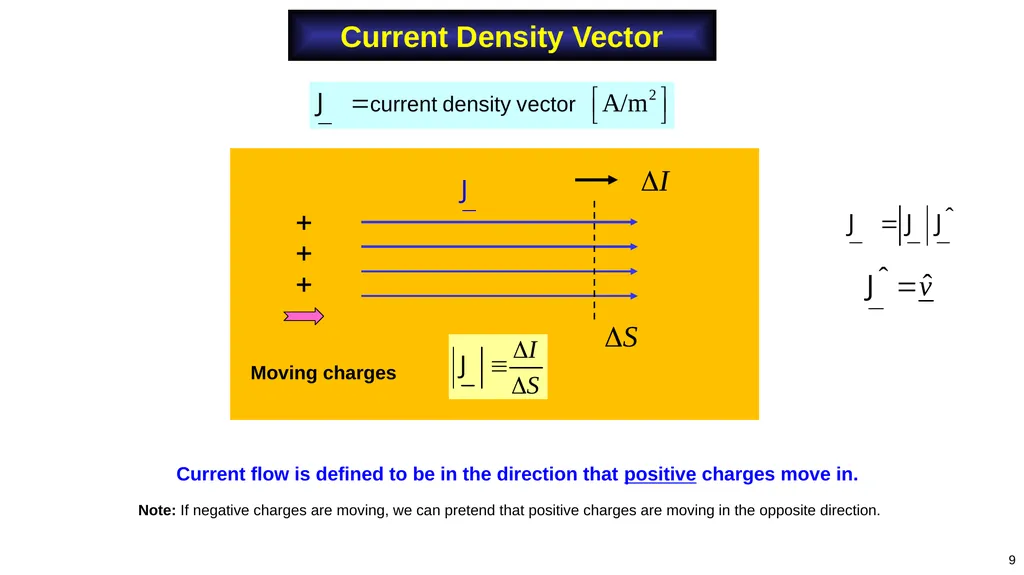
Current Density Vector 9 Current flow is defined to be in the direction that positive charges move in. Note: If negative charges are moving, we can pretend that positive charges are moving in the opposite direction.<br>
10
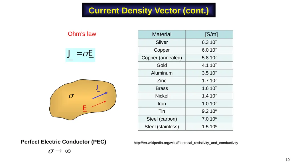
Current Density Vector (cont.) 10 http://en.wikipedia.org/wiki/Electrical_resistivity_and_conductivity Ohm’s law Perfect Electric Conductor (PEC)<br>
11
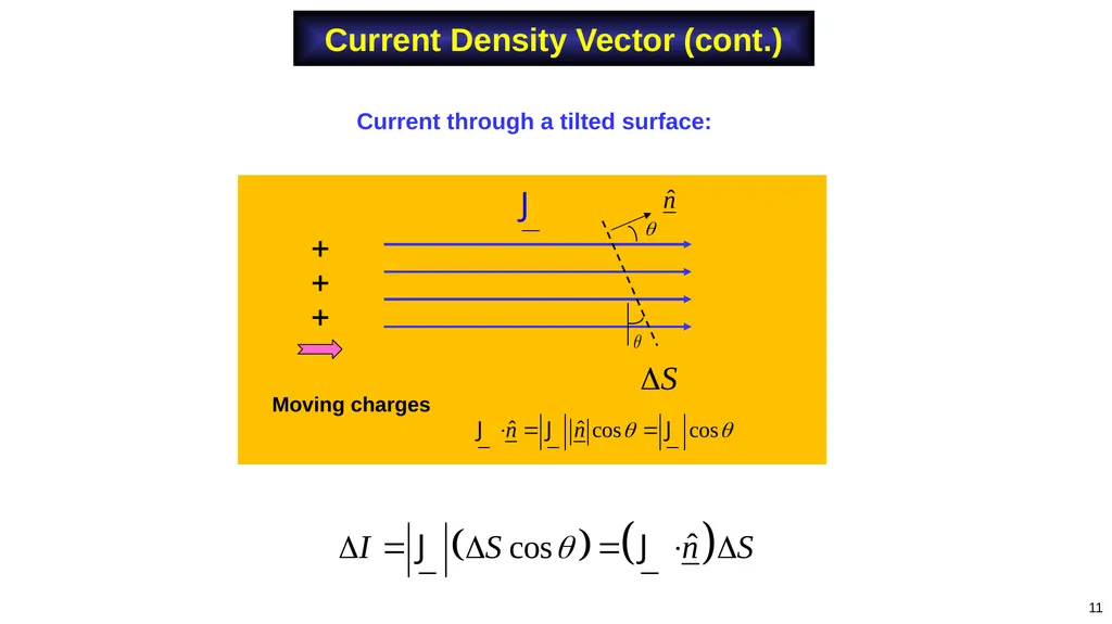
11 Current through a tilted surface: Current Density Vector (cont.) Moving charges<br>
12
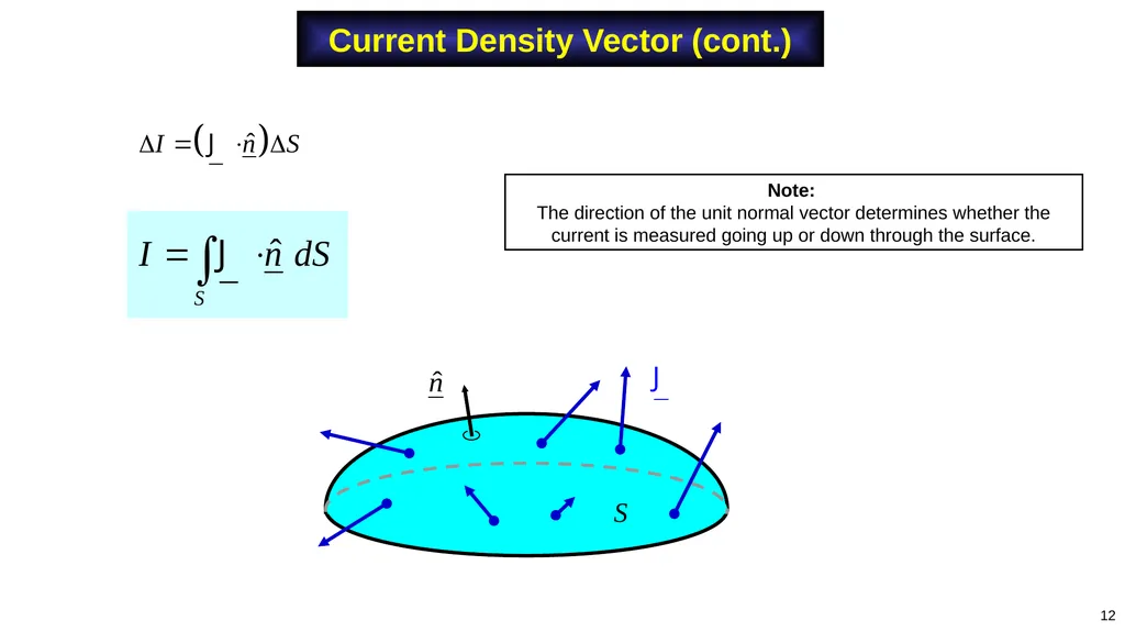
Current Density Vector (cont.) 12 Note:
The direction of the unit normal vector determines whether the current is measured going up or down through the surface.<br>
The direction of the unit normal vector determines whether the current is measured going up or down through the surface.<br>
13
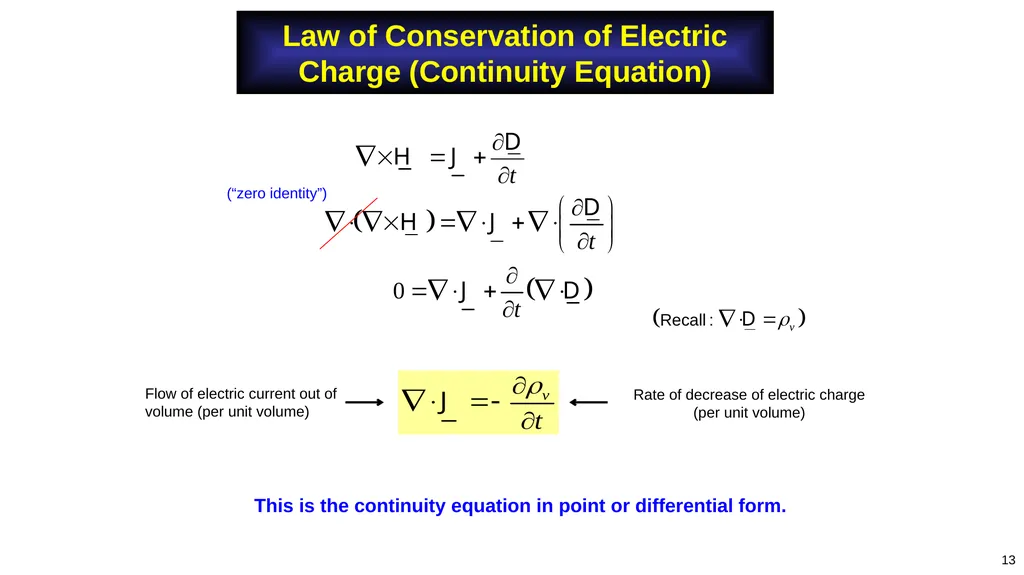
Law of Conservation of Electric Charge (Continuity Equation) Flow of electric current out of volume (per unit volume) Rate of decrease of electric charge (per unit volume) 13 This is the continuity equation in point or differential form. (“zero identity”)<br>
14
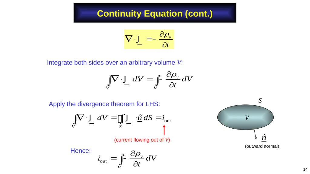
Continuity Equation (cont.) Apply the divergence theorem for LHS: Integrate both sides over an arbitrary volume V: 14 Hence: (current flowing out of V)<br>
15
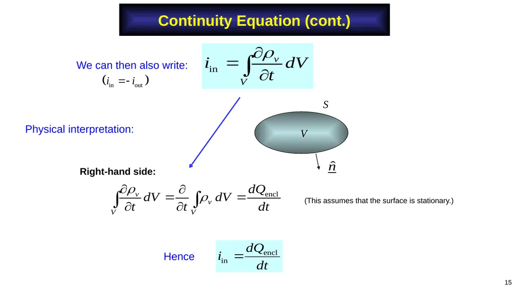
Continuity Equation (cont.) Physical interpretation: (This assumes that the surface is stationary.) 15 Hence Right-hand side: We can then also write:<br>
16
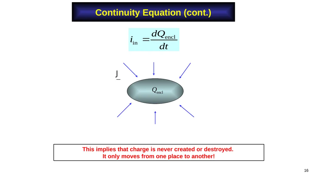
Continuity Equation (cont.) 16 This implies that charge is never created or destroyed.
It only moves from one place to another!<br>
It only moves from one place to another!<br>
17
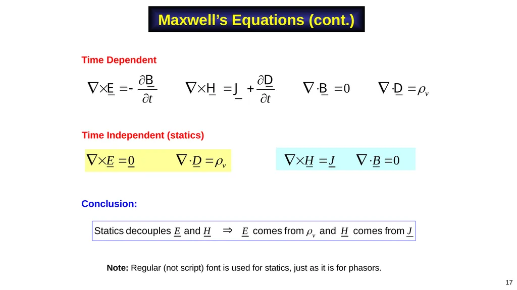
17 Maxwell’s Equations (cont.) Note: Regular (not script) font is used for statics, just as it is for phasors. Time Dependent Time Independent (statics) Conclusion:<br>
18
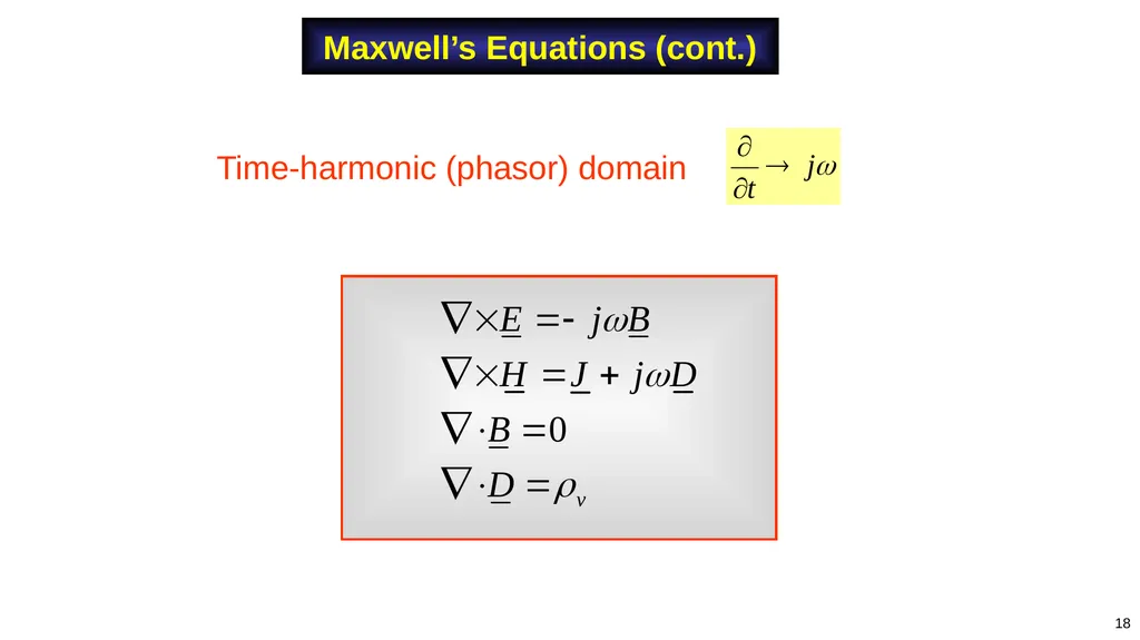
Time-harmonic (phasor) domain 18 Maxwell’s Equations (cont.)<br>
19
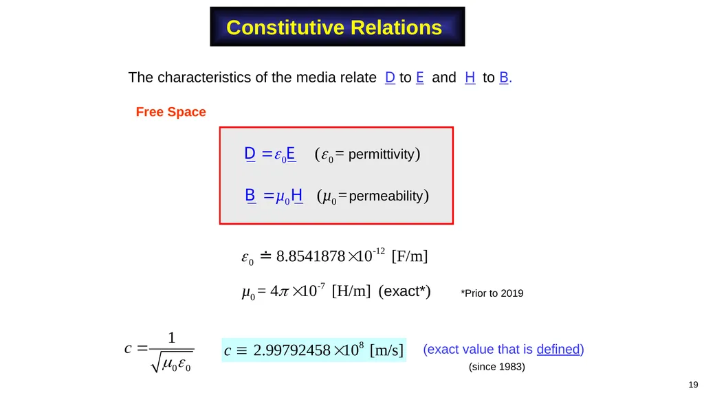
Constitutive Relations The characteristics of the media relate D to E and H to B. (exact value that is defined) Free Space 19 *Prior to 2019 (since 1983)<br>
20
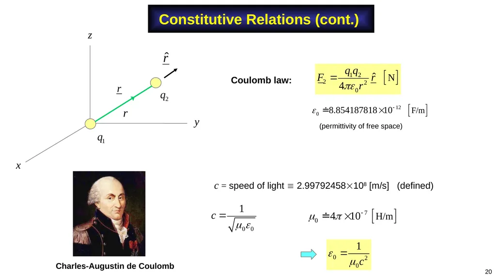
Constitutive Relations (cont.) 20 Experimental law: c = speed of light 2.99792458108 [m/s] (defined) Charles-Augustin de Coulomb Here is how we can calculate 0 accurately: (permittivity of free space) Coulomb law:<br>
21
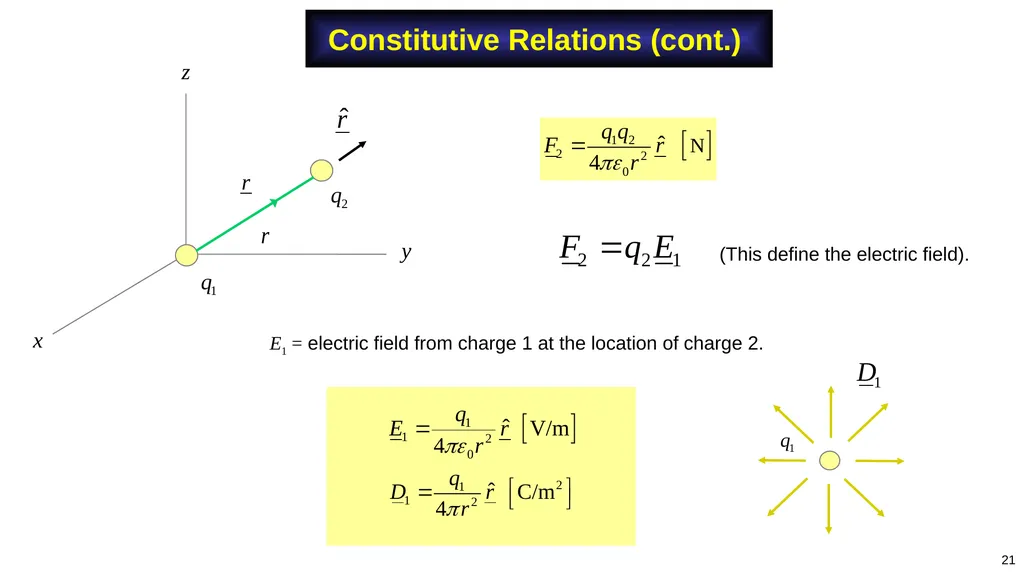
Constitutive Relations (cont.) 21 Experimental law: E1 = electric field from charge 1 at the location of charge 2. (This define the electric field).<br>
22
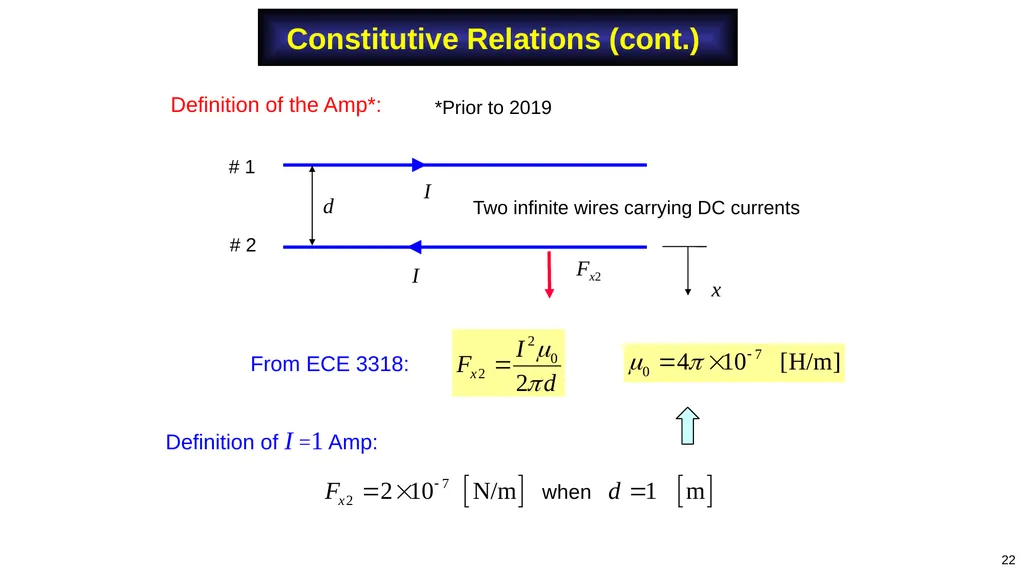
22 Definition of I =1 Amp: Definition of the Amp*: From ECE 3318: Constitutive Relations (cont.) *Prior to 2019<br>
23
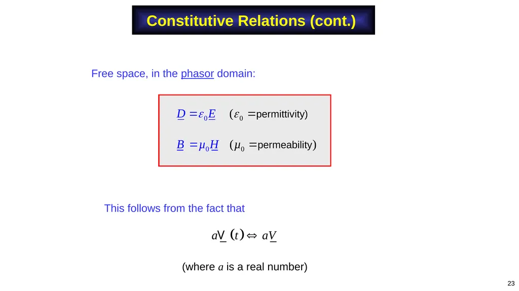
Constitutive Relations (cont.) Free space, in the phasor domain: This follows from the fact that (where a is a real number) 23<br>
24
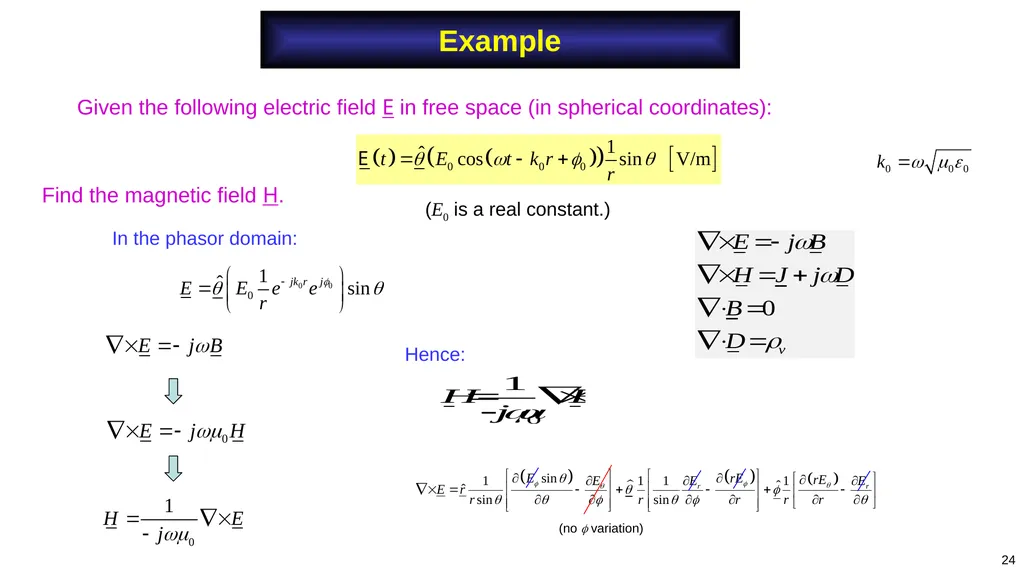
Example Given the following electric field E in free space (in spherical coordinates): 24 Find the magnetic field H. In the phasor domain: Hence: (no variation) (E0 is a real constant.)<br>
25
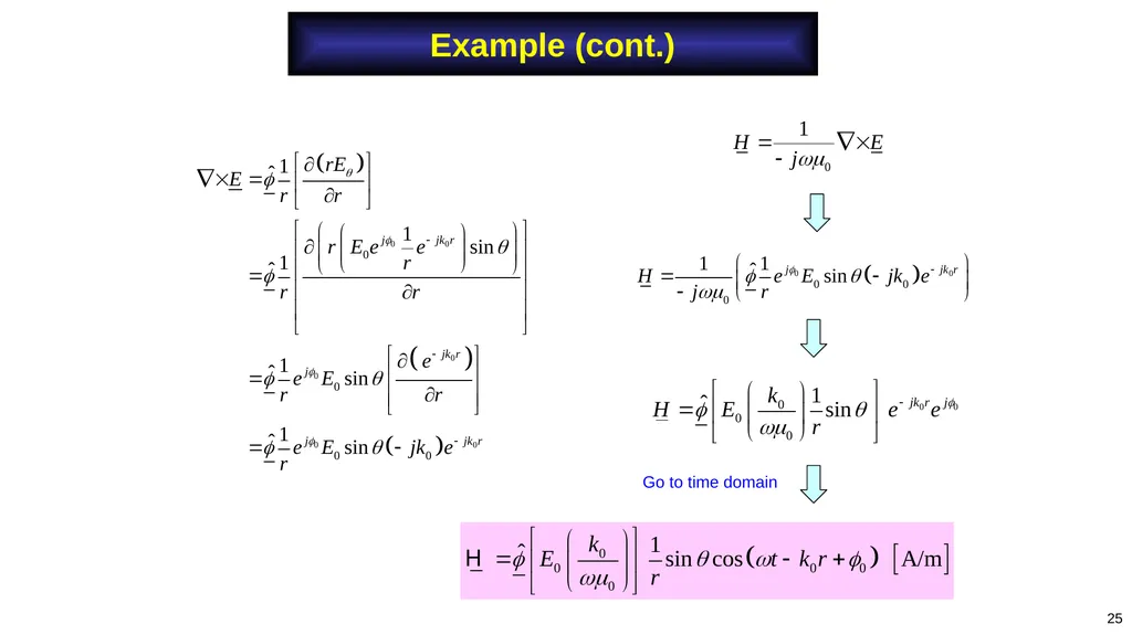
Example (cont.) 25 Go to time domain<br>
26
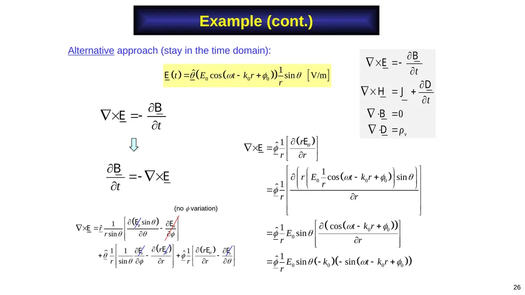
Example (cont.) 26 Alternative approach (stay in the time domain): (no variation)<br>
27
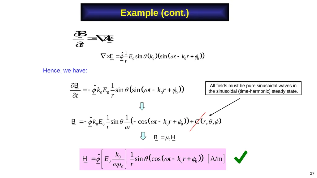
Example (cont.) 27 Hence, we have: All fields must be pure sinusoidal waves in the sinusoidal (time-harmonic) steady state.<br>
28
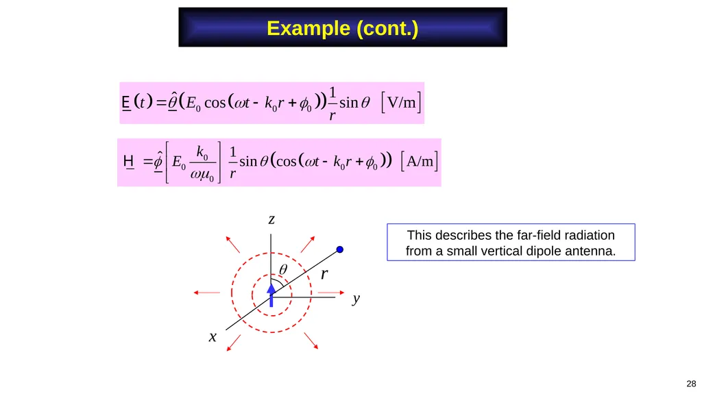
Example (cont.) 28 This describes the far-field radiation from a small vertical dipole antenna.<br>
29
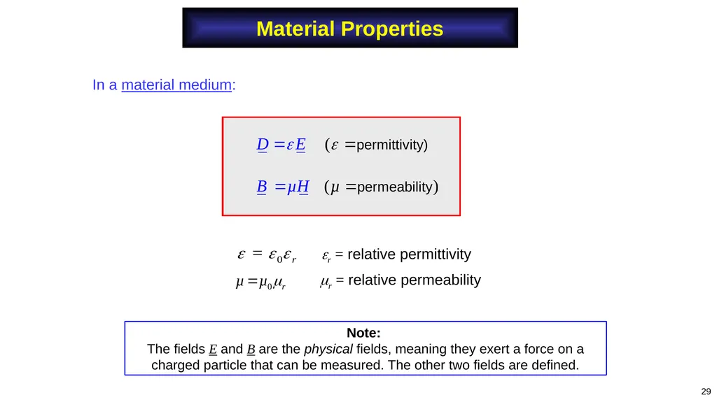
In a material medium: r = relative permittivity r = relative permeability 29 Material Properties Note:
The fields E and B are the physical fields, meaning they exert a force on a charged particle that can be measured. The other two fields are defined.<br>
The fields E and B are the physical fields, meaning they exert a force on a charged particle that can be measured. The other two fields are defined.<br>
30
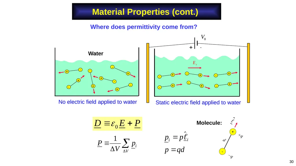
30 Material Properties (cont.) Where does permittivity come from? Water Molecule: Static electric field applied to water No electric field applied to water<br>
31
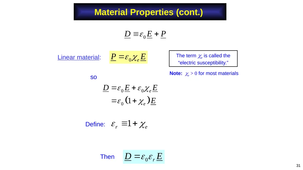
31 Linear material: Define: Then Note: e > 0 for most materials The term e is called the “electric susceptibility.” so Material Properties (cont.)<br>
32
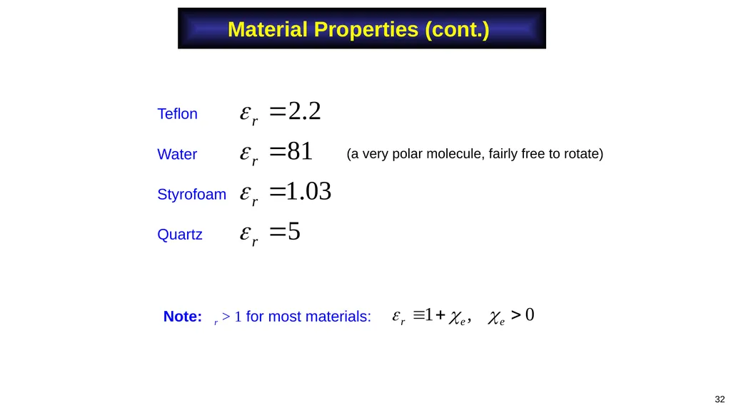
32 Teflon
Water
Styrofoam
Quartz (a very polar molecule, fairly free to rotate) Note: r > 1 for most materials: Material Properties (cont.)<br>
Water
Styrofoam
Quartz (a very polar molecule, fairly free to rotate) Note: r > 1 for most materials: Material Properties (cont.)<br>
33
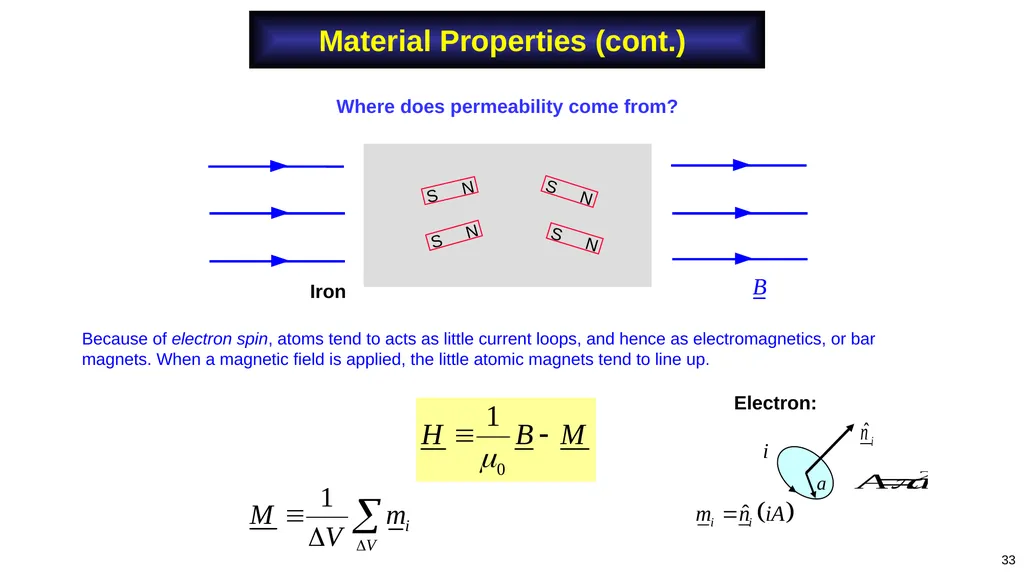
33 Where does permeability come from? Because of electron spin, atoms tend to acts as little current loops, and hence as electromagnetics, or bar magnets. When a magnetic field is applied, the little atomic magnets tend to line up. Material Properties (cont.) Iron<br>
34
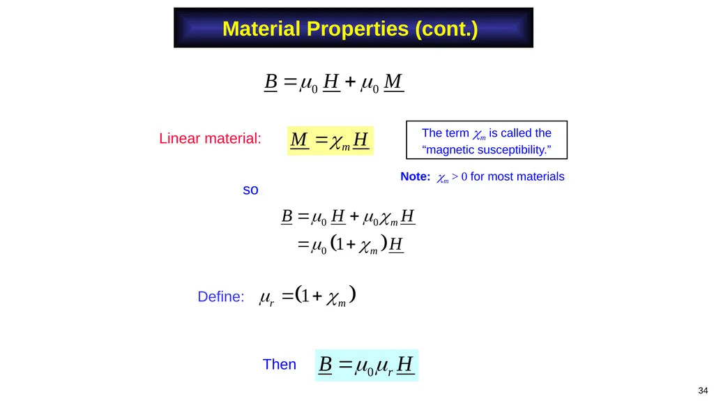
34 so Define: Then The term m is called the “magnetic susceptibility.” Linear material: Note: m > 0 for most materials Material Properties (cont.)<br>
35
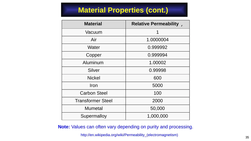
35 Note: Values can often vary depending on purity and processing. http://en.wikipedia.org/wiki/Permeability_(electromagnetism) Material Properties (cont.)<br>
36
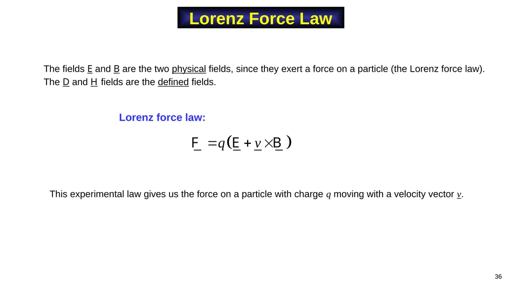
Lorenz Force Law 36 The fields E and B are the two physical fields, since they exert a force on a particle (the Lorenz force law). The D and H fields are the defined fields. Lorenz force law: This experimental law gives us the force on a particle with charge q moving with a velocity vector v.<br>
37
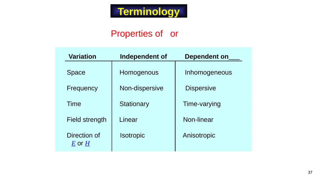
Variation Independent of Dependent on
Space Homogenous Inhomogeneous
Frequency Non-dispersive Dispersive
Time Stationary Time-varying
Field strength Linear Non-linear
Direction of Isotropic Anisotropic
E or H Terminology 37 Properties of or <br>
Space Homogenous Inhomogeneous
Frequency Non-dispersive Dispersive
Time Stationary Time-varying
Field strength Linear Non-linear
Direction of Isotropic Anisotropic
E or H Terminology 37 Properties of or <br>
38
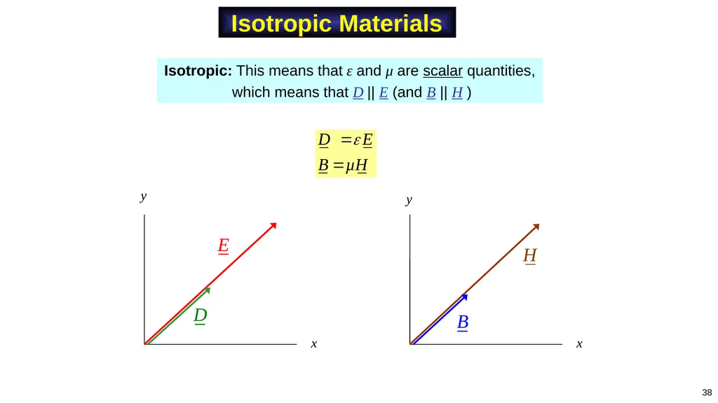
Isotropic Materials Isotropic: This means that ε and μ are scalar quantities,
which means that D || E (and B || H ) 38<br>
which means that D || E (and B || H ) 38<br>
39
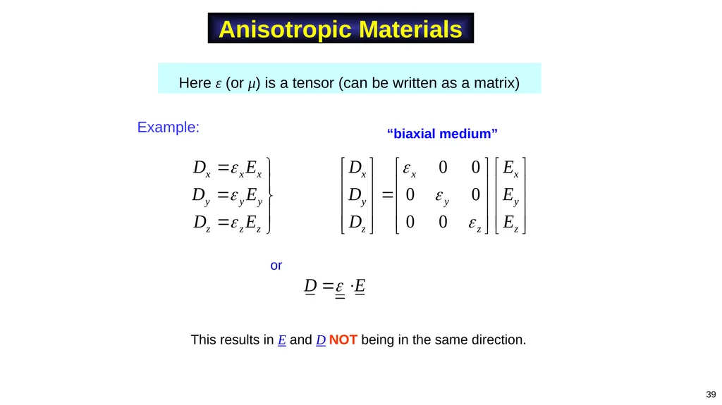
Here ε (or μ) is a tensor (can be written as a matrix) This results in E and D NOT being in the same direction. Anisotropic Materials 39 Example: or “biaxial medium”<br>
40
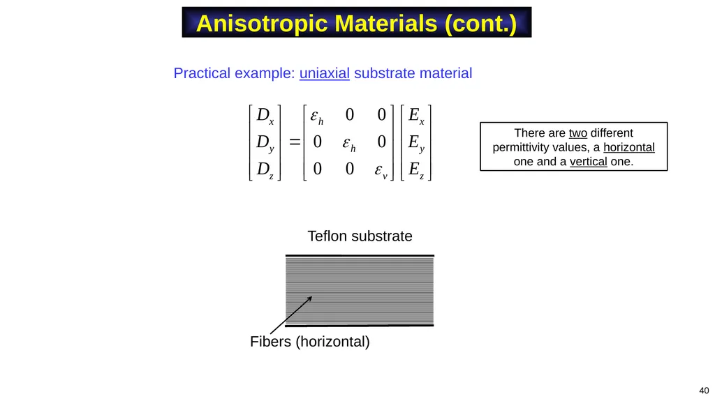
Anisotropic Materials (cont.) 40 Practical example: uniaxial substrate material There are two different permittivity values, a horizontal one and a vertical one.<br>
41
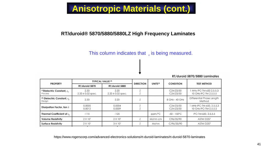
Anisotropic Materials (cont.) 41 This column indicates that v is being measured. RT/duroid® 5870/5880/5880LZ High Frequency Laminates https://www.rogerscorp.com/advanced-electronics-solutions/rt-duroid-laminates/rt-duroid-5870-laminates<br>