
Adaptive control an adaptive controller is thus a
Description: Adaptive control an adaptive controller is thus a controller that can modify its behavior in response to changes in the dynamics of the process and the character of the disturbances. an adaptive controller is a controller with adjustable
Related Topics
Download Presentation
"Adaptive control an adaptive controller is thus a" is the property of its rightful owner. Permission is granted to download and print the materials on this website for personal, non-commercial use only, and to display it on your personal computer provided you do not modify the materials and that you retain all copyright notices contained in the materials. By downloading content from our website, you accept the terms of this agreement.
Presentation Transcript
slide1. Adaptive control an adaptive controller is thus a controller that
can modify its behavior in response to changes in the dynamics of the process and the character of the disturbances.
an adaptive controller is a controller with adjustable parameters and a mechanism for adjusting the parameters. The controller becomes nonlinear because of the parameter
adjustment .
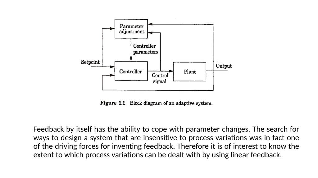
An adaptive control system can be thought of as having two loops. One loop is a normal feedback with the process and the controller. The other loop is the parameter adjustment loop.
A block diagram of an adaptive system is shown in Fig. 1.1. The parameter adjustment loop is often slower than the normal feedback loop.<br>
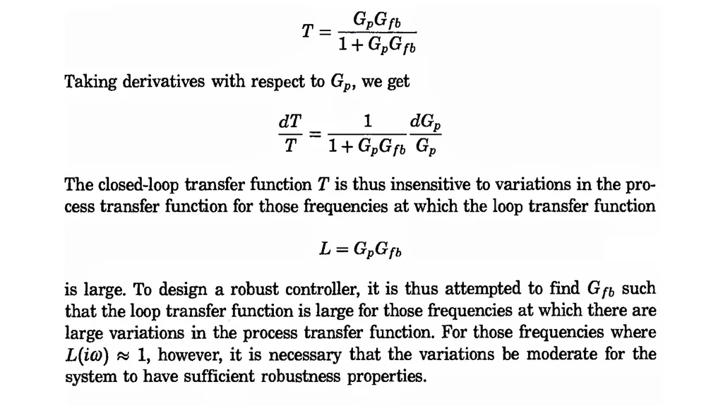
slide2. Feedback by itself has the ability to cope with parameter changes. The search for ways to design a system that are insensitive to process variations was in fact one of the driving forces for inventing feedback. Therefore it is of interest to know the extent to which process variations can be dealt with by using linear feedback.<br>
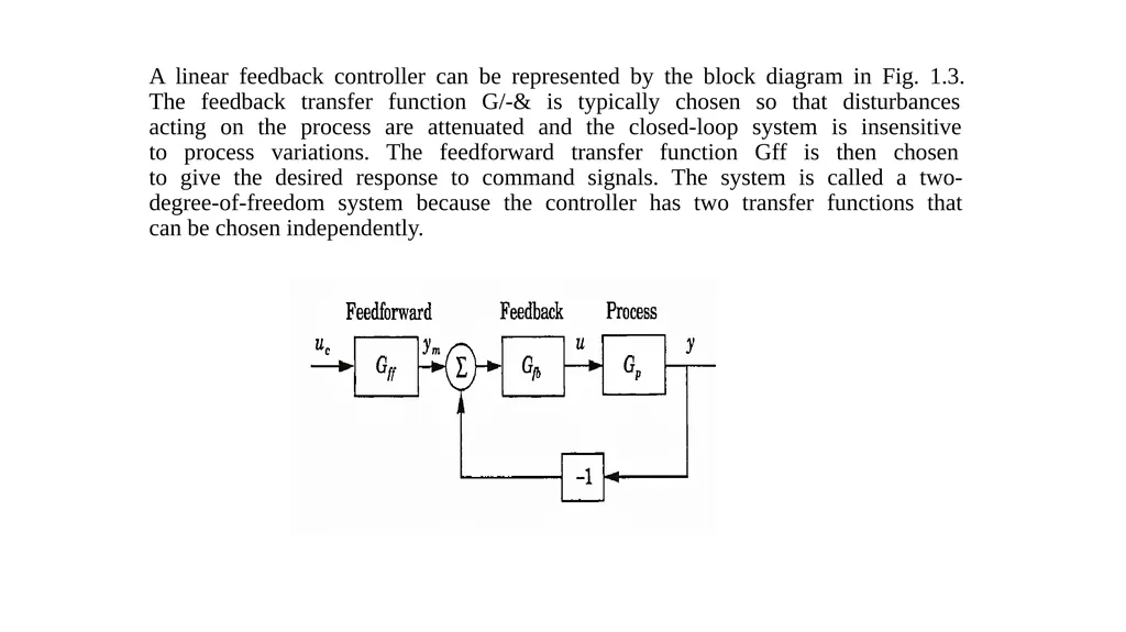
slide3. A linear feedback controller can be represented by the block diagram in Fig. 1.3. The feedback transfer function G/-& is typically chosen so that disturbances acting on the process are attenuated and the closed-loop system is insensitive to process variations. The feedforward transfer function Gff is then chosen to give the desired response to command signals. The system is called a two- degree-of-freedom system because the controller has two transfer functions that can be chosen independently.<br>
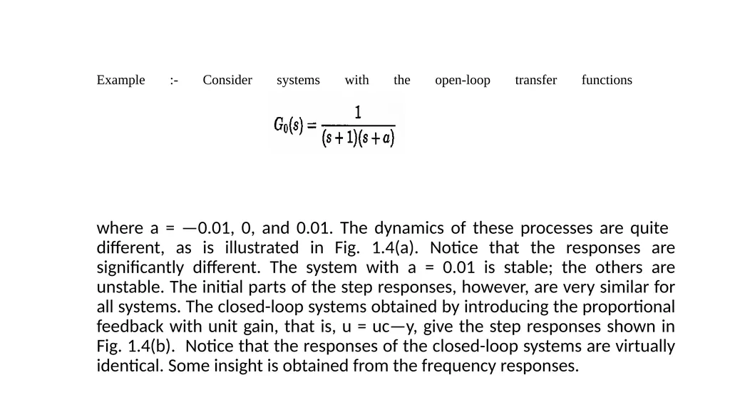
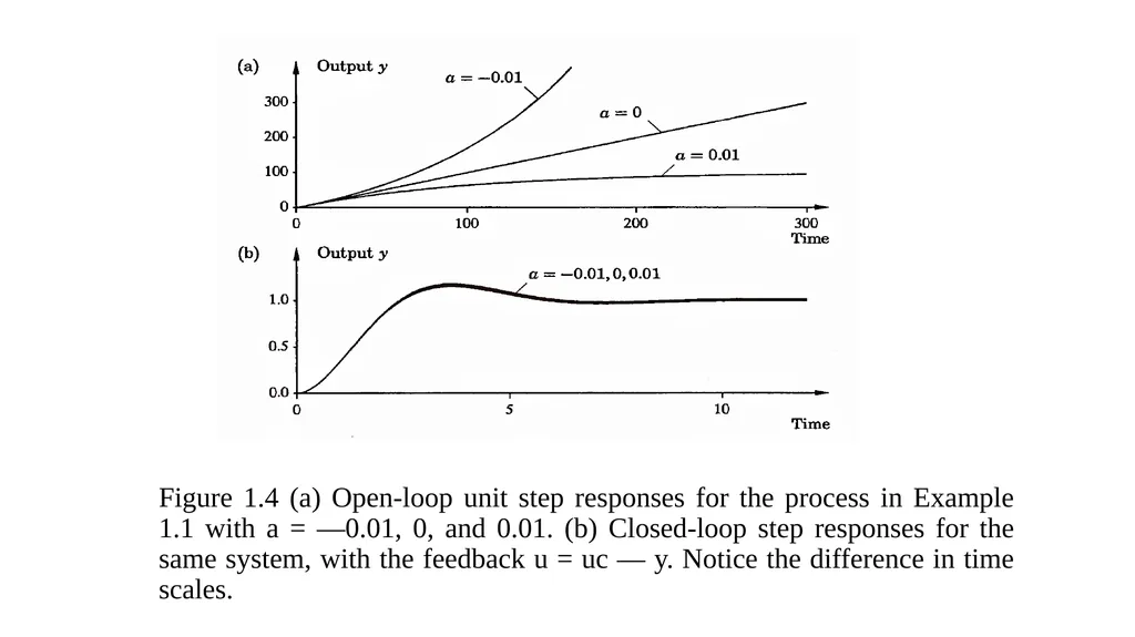
slide5. Example :- Consider systems with the open-loop transfer functions where a = —0.01, 0, and 0.01. The dynamics of these processes are quite different, as is illustrated in Fig. 1.4(a). Notice that the responses are significantly different. The system with a = 0.01 is stable; the others are unstable. The initial parts of the step responses, however, are very similar for all systems. The closed-loop systems obtained by introducing the proportional feedback with unit gain, that is, u = uc—y, give the step responses shown in Fig. 1.4(b). Notice that the responses of the closed-loop systems are virtually identical. Some insight is obtained from the frequency responses.<br>
slide6. Figure 1.4 (a) Open-loop unit step responses for the process in Example 1.1 with a = —0.01, 0, and 0.01. (b) Closed-loop step responses for the same system, with the feedback u = uc — y. Notice the difference in time scales.<br>
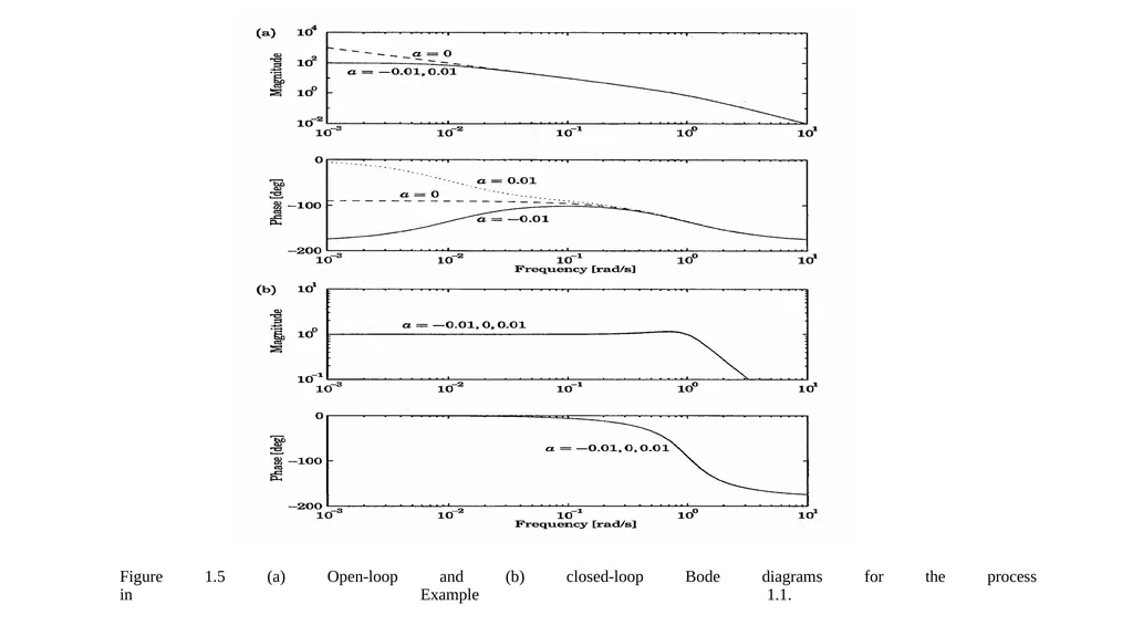
slide7. Figure 1.5 (a) Open-loop and (b) closed-loop Bode diagrams for the process in Example 1.1.<br>
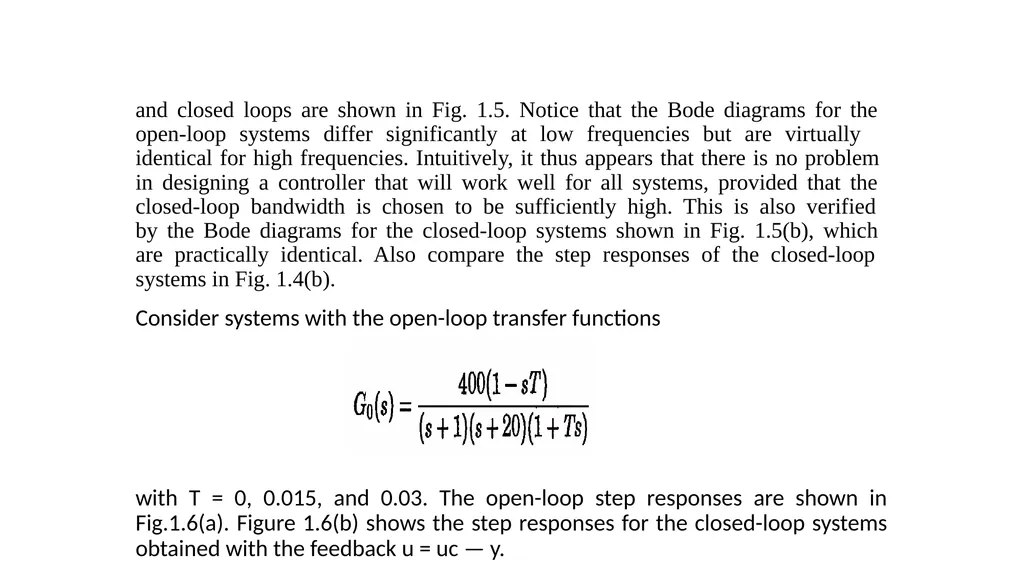
slide8. and closed loops are shown in Fig. 1.5. Notice that the Bode diagrams for the open-loop systems differ significantly at low frequencies but are virtually identical for high frequencies. Intuitively, it thus appears that there is no problem in designing a controller that will work well for all systems, provided that the closed-loop bandwidth is chosen to be sufficiently high. This is also verified by the Bode diagrams for the closed-loop systems shown in Fig. 1.5(b), which are practically identical. Also compare the step responses of the closed-loop systems in Fig. 1.4(b). Consider systems with the open-loop transfer functions
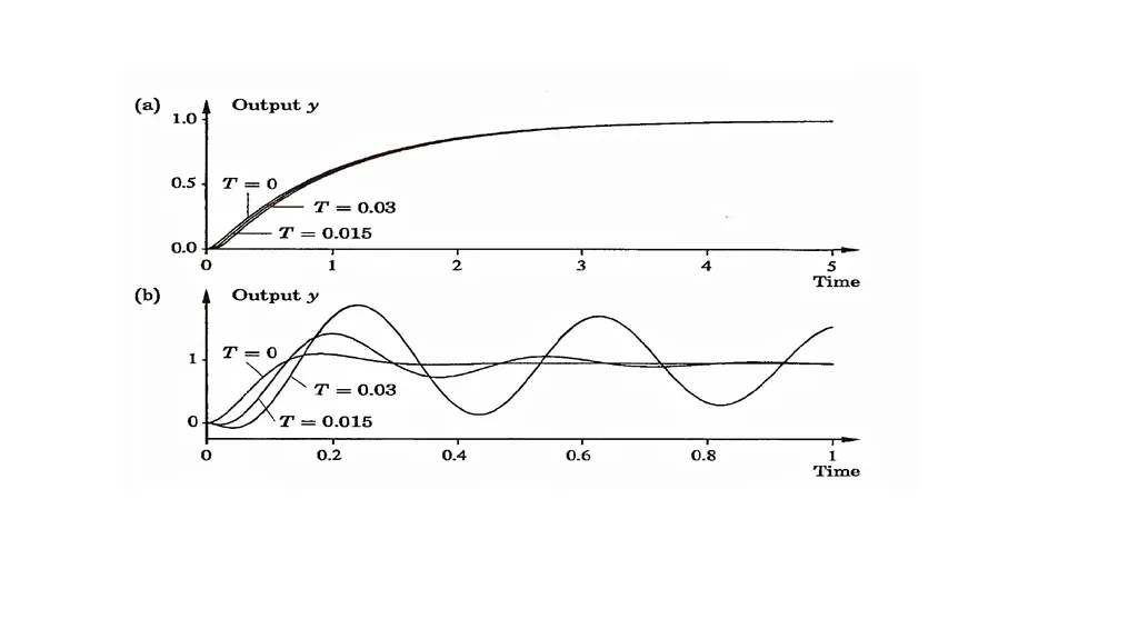
with T = 0, 0.015, and 0.03. The open-loop step responses are shown in Fig.1.6(a). Figure 1.6(b) shows the step responses for the closed-loop systems obtained with the feedback u = uc — y.<br>
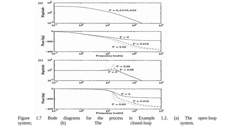
slide10. Notice that the open-loop responses are very similar but that the closed-loop responses differ considerably. The frequency responses give some insight. The Bode diagrams for the open- and closed-loop systems are shown in Fig. 1.7. Notice that the frequency responses of the open-loop systems are very close for low frequencies but differ considerably in the phase at high frequencies. It is thus possible to design a controller that works well for all systems provided that the closed-loop bandwidth is chosen to be sufficiently small. At the crossover frequency chosen in the example there are, however, significant variations that show up in the Bode diagrams of the closed-loop systems in Fig. 1.7(b) and in the step responses of the closed-loop system in Fig. 1.6(b).<br>
slide11. Figure 1.7 Bode diagrams for the process in Example 1.2. (a) The open-loop system; (b) The closed-loop system.<br>
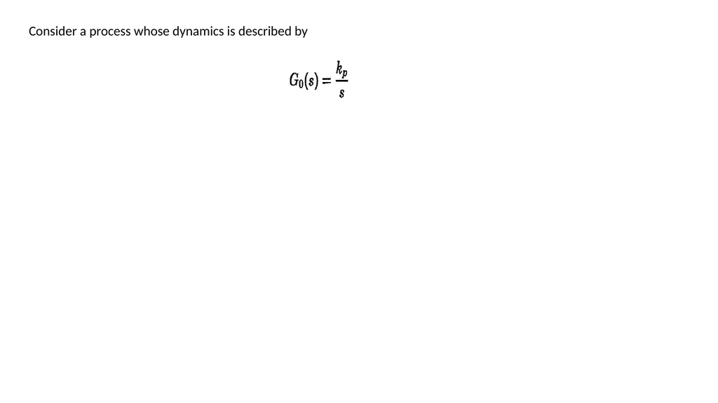
slide12. Consider a process whose dynamics is described by<br>
an adaptive controller is a controller with adjustable parameters and a mechanism for adjusting the parameters. The controller becomes nonlinear because of the parameter
adjustment .
An adaptive control system can be thought of as having two loops. One loop is a normal feedback with the process and the controller. The other loop is the parameter adjustment loop.
A block diagram of an adaptive system is shown in Fig. 1.1. The parameter adjustment loop is often slower than the normal feedback loop.<br>
slide2. Feedback by itself has the ability to cope with parameter changes. The search for ways to design a system that are insensitive to process variations was in fact one of the driving forces for inventing feedback. Therefore it is of interest to know the extent to which process variations can be dealt with by using linear feedback.<br>
slide3. A linear feedback controller can be represented by the block diagram in Fig. 1.3. The feedback transfer function G/-& is typically chosen so that disturbances acting on the process are attenuated and the closed-loop system is insensitive to process variations. The feedforward transfer function Gff is then chosen to give the desired response to command signals. The system is called a two- degree-of-freedom system because the controller has two transfer functions that can be chosen independently.<br>
slide5. Example :- Consider systems with the open-loop transfer functions where a = —0.01, 0, and 0.01. The dynamics of these processes are quite different, as is illustrated in Fig. 1.4(a). Notice that the responses are significantly different. The system with a = 0.01 is stable; the others are unstable. The initial parts of the step responses, however, are very similar for all systems. The closed-loop systems obtained by introducing the proportional feedback with unit gain, that is, u = uc—y, give the step responses shown in Fig. 1.4(b). Notice that the responses of the closed-loop systems are virtually identical. Some insight is obtained from the frequency responses.<br>
slide6. Figure 1.4 (a) Open-loop unit step responses for the process in Example 1.1 with a = —0.01, 0, and 0.01. (b) Closed-loop step responses for the same system, with the feedback u = uc — y. Notice the difference in time scales.<br>
slide7. Figure 1.5 (a) Open-loop and (b) closed-loop Bode diagrams for the process in Example 1.1.<br>
slide8. and closed loops are shown in Fig. 1.5. Notice that the Bode diagrams for the open-loop systems differ significantly at low frequencies but are virtually identical for high frequencies. Intuitively, it thus appears that there is no problem in designing a controller that will work well for all systems, provided that the closed-loop bandwidth is chosen to be sufficiently high. This is also verified by the Bode diagrams for the closed-loop systems shown in Fig. 1.5(b), which are practically identical. Also compare the step responses of the closed-loop systems in Fig. 1.4(b). Consider systems with the open-loop transfer functions
with T = 0, 0.015, and 0.03. The open-loop step responses are shown in Fig.1.6(a). Figure 1.6(b) shows the step responses for the closed-loop systems obtained with the feedback u = uc — y.<br>
slide10. Notice that the open-loop responses are very similar but that the closed-loop responses differ considerably. The frequency responses give some insight. The Bode diagrams for the open- and closed-loop systems are shown in Fig. 1.7. Notice that the frequency responses of the open-loop systems are very close for low frequencies but differ considerably in the phase at high frequencies. It is thus possible to design a controller that works well for all systems provided that the closed-loop bandwidth is chosen to be sufficiently small. At the crossover frequency chosen in the example there are, however, significant variations that show up in the Bode diagrams of the closed-loop systems in Fig. 1.7(b) and in the step responses of the closed-loop system in Fig. 1.6(b).<br>
slide11. Figure 1.7 Bode diagrams for the process in Example 1.2. (a) The open-loop system; (b) The closed-loop system.<br>
slide12. Consider a process whose dynamics is described by<br>