
Aggregate Supply and the Short-Run Tradeoff
YM
Published · 34 slides · 0 views

1 / 1


Description
Aggregate Supply and the Short-Run Tradeoff Between Inflation and Unemployment Macroeconomics N. Gregory Mankiw 2019 Worth Publishers, all rights reserved IN THIS CHAPTER, YOU WILL LEARN: About two models of aggregate supply in which
Related Topics
Share
Embed code
Download this presentation From Below
"Aggregate Supply and the Short-Run Tradeoff" is the property of its rightful owner. Permission is granted to download and print the materials on this website for personal, non-commercial use only, and to display it on your personal computer provided you do not modify the materials and that you retain all copyright notices contained in the materials. By downloading content from our website, you accept the terms of this agreement.
Presentation Transcript
01
Aggregate Supply and the Short-Run Tradeoff Between Inflation and Unemployment Macroeconomics
N. Gregory Mankiw © 2019 Worth Publishers, all rights reserved<br>
N. Gregory Mankiw © 2019 Worth Publishers, all rights reserved<br>
02
IN THIS CHAPTER, YOU WILL LEARN: About two models of aggregate supply in which output depends positively on the price level in the short run
About the short-run tradeoff between inflation and unemployment, known as the Phillips curve<br>
About the short-run tradeoff between inflation and unemployment, known as the Phillips curve<br>
03
Introduction, part 1 In previous chapters, we assumed that the price level P was “stuck” in the short run.
This implies a horizontal SRAS curve.
Now, we consider two prominent models of aggregate supply in the short run:
Sticky-price model
Imperfect-information model<br>
This implies a horizontal SRAS curve.
Now, we consider two prominent models of aggregate supply in the short run:
Sticky-price model
Imperfect-information model<br>
04
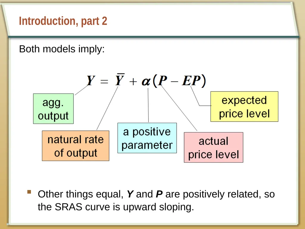
Introduction, part 2 Both models imply: Other things equal, Y and P are positively related, so the SRAS curve is upward sloping.<br>
05
The sticky-price model, part 1 Reasons for sticky prices:
long-term contracts between firms and customers
menu costs
firms not wishing to annoy customers with frequent price changes
Assumption:
Firms set their own prices (as in monopolistic competition).<br>
long-term contracts between firms and customers
menu costs
firms not wishing to annoy customers with frequent price changes
Assumption:
Firms set their own prices (as in monopolistic competition).<br>
06
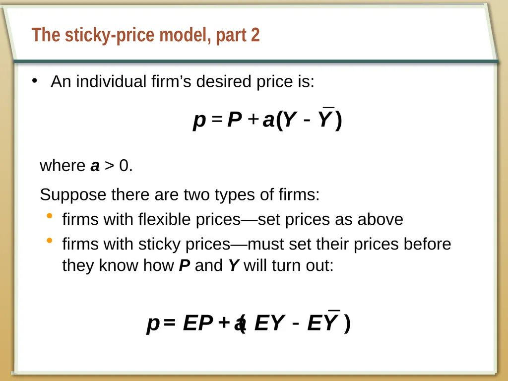
The sticky-price model, part 2 An individual firm’s desired price is: where a > 0.
Suppose there are two types of firms:
firms with flexible prices—set prices as above
firms with sticky prices—must set their prices before they know how P and Y will turn out:<br>
Suppose there are two types of firms:
firms with flexible prices—set prices as above
firms with sticky prices—must set their prices before they know how P and Y will turn out:<br>
07
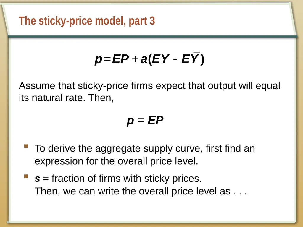
The sticky-price model, part 3 Assume that sticky-price firms expect that output will equal its natural rate. Then, To derive the aggregate supply curve, first find an expression for the overall price level.
s = fraction of firms with sticky prices. Then, we can write the overall price level as . . .<br>
s = fraction of firms with sticky prices. Then, we can write the overall price level as . . .<br>
08
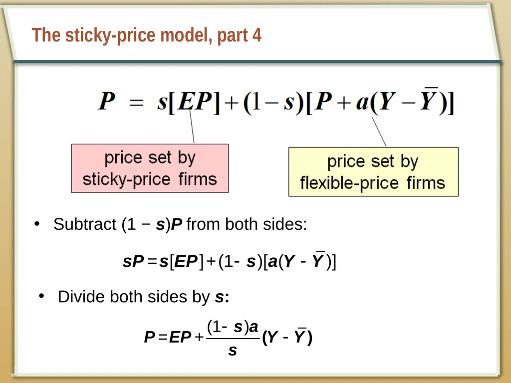
The sticky-price model, part 4 Subtract (1 − s)P from both sides: Divide both sides by s:<br>
09
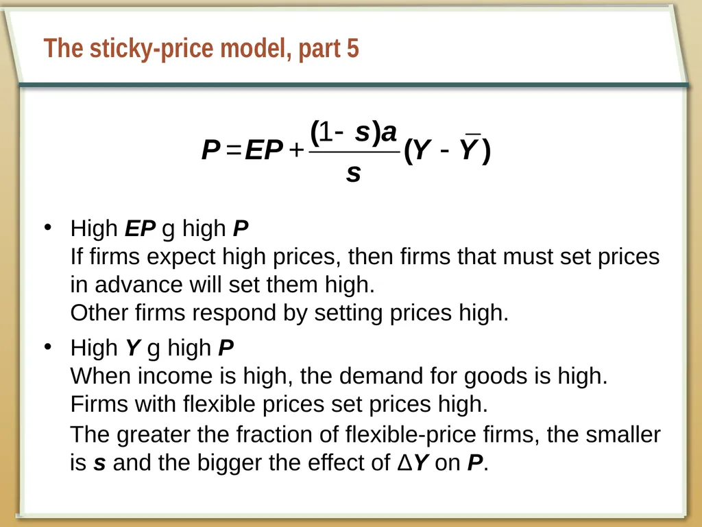
The sticky-price model, part 5 High EP g high P
If firms expect high prices, then firms that must set prices in advance will set them high.
Other firms respond by setting prices high.
High Y g high P When income is high, the demand for goods is high. Firms with flexible prices set prices high.
The greater the fraction of flexible-price firms, the smaller is s and the bigger the effect of ΔY on P.<br>
High Y g high P When income is high, the demand for goods is high. Firms with flexible prices set prices high.
The greater the fraction of flexible-price firms, the smaller is s and the bigger the effect of ΔY on P.<br>
10
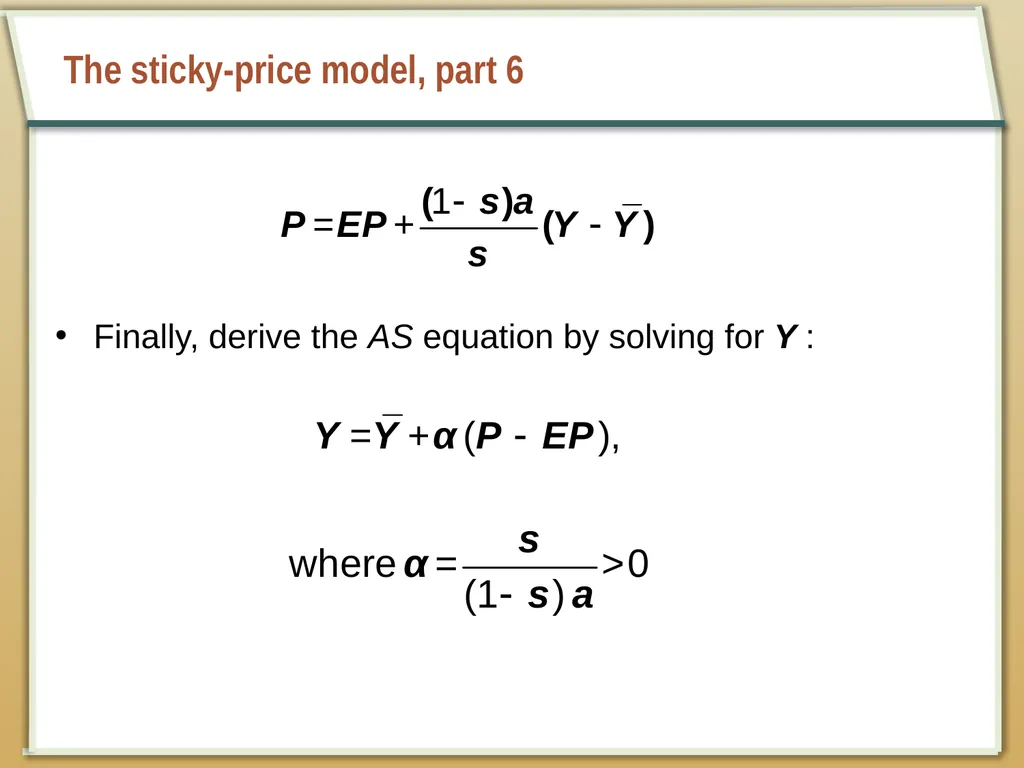
The sticky-price model, part 6 Finally, derive the AS equation by solving for Y :<br>
11
The imperfect-information model, part 1 Assumptions:
All wages and prices are perfectly flexible, and all markets are clear.
Each supplier produces one good and consumes many goods.
Each supplier knows the nominal price of the good she produces but does not know the overall price level.<br>
All wages and prices are perfectly flexible, and all markets are clear.
Each supplier produces one good and consumes many goods.
Each supplier knows the nominal price of the good she produces but does not know the overall price level.<br>
12
The imperfect-information model, part 2 The supply of each good depends on its relative price: the nominal price of the good divided by the overall price level.
The supplier doesn’t know price level at the time she makes her production decision so uses EP.
Suppose P rises but EP does not.
Supplier thinks her relative price has risen, so she produces more.
With many producers thinking this way, Y will rise whenever P rises above EP.<br>
The supplier doesn’t know price level at the time she makes her production decision so uses EP.
Suppose P rises but EP does not.
Supplier thinks her relative price has risen, so she produces more.
With many producers thinking this way, Y will rise whenever P rises above EP.<br>
13
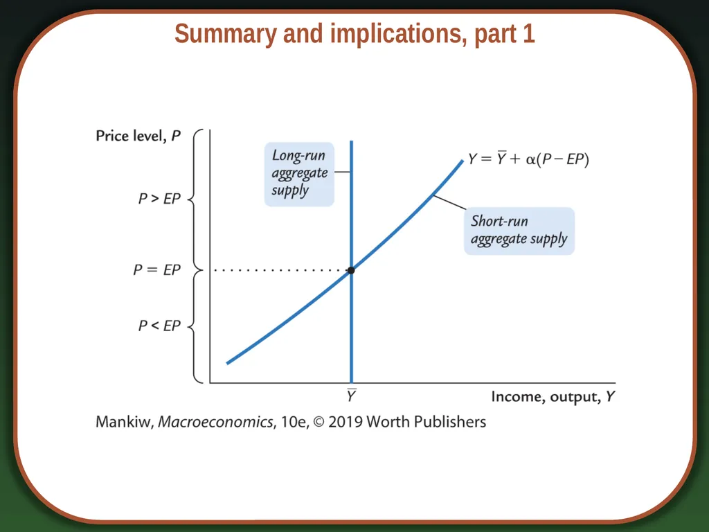
Summary and implications, part 1<br>
14
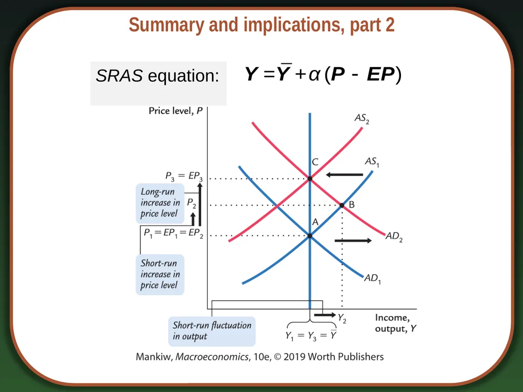
Summary and implications, part 2 SRAS equation:<br>
15
Inflation, unemployment, and the Phillips curve The Phillips curve states that π depends on:
expected inflation, Eπ
cyclical unemployment: the deviation of the actual rate of unemployment (u) from the natural rate (un)
supply shocks, ν (Greek letter nu). where β > 0 is an exogenous constant.<br>
expected inflation, Eπ
cyclical unemployment: the deviation of the actual rate of unemployment (u) from the natural rate (un)
supply shocks, ν (Greek letter nu). where β > 0 is an exogenous constant.<br>
16
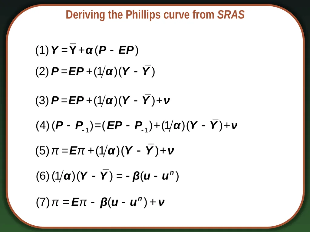
Deriving the Phillips curve from SRAS<br>
17
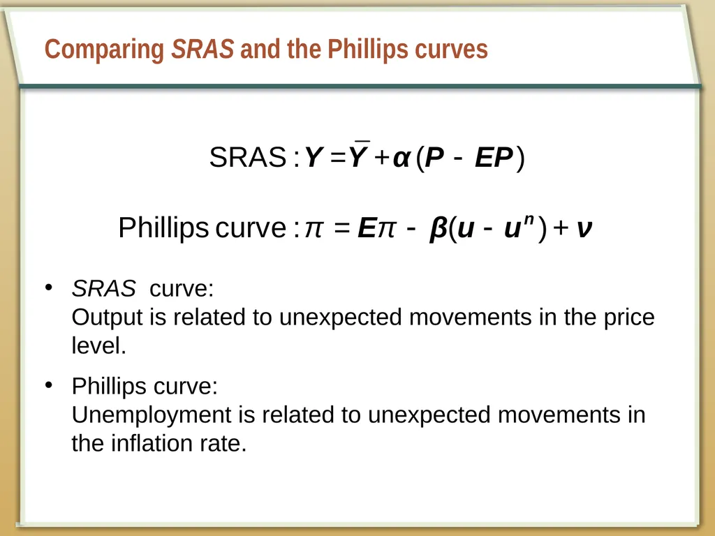
Comparing SRAS and the Phillips curves SRAS curve:
Output is related to unexpected movements in the price level.
Phillips curve: Unemployment is related to unexpected movements in the inflation rate.<br>
Phillips curve: Unemployment is related to unexpected movements in the inflation rate.<br>
18
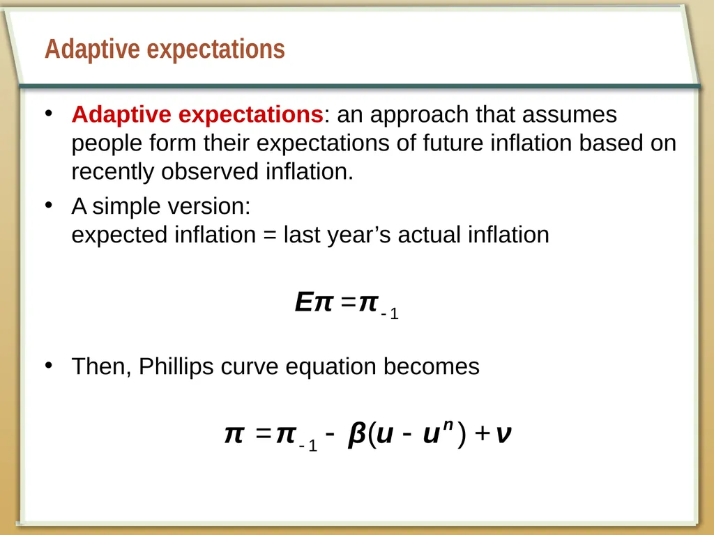
Adaptive expectations Adaptive expectations: an approach that assumes people form their expectations of future inflation based on recently observed inflation.
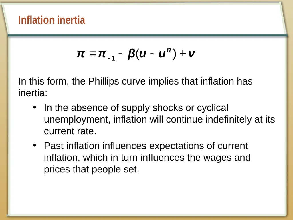
A simple version: expected inflation = last year’s actual inflation Then, Phillips curve equation becomes<br>
A simple version: expected inflation = last year’s actual inflation Then, Phillips curve equation becomes<br>
19
Inflation inertia In this form, the Phillips curve implies that inflation has inertia:
In the absence of supply shocks or cyclical unemployment, inflation will continue indefinitely at its current rate.
Past inflation influences expectations of current inflation, which in turn influences the wages and prices that people set.<br>
In the absence of supply shocks or cyclical unemployment, inflation will continue indefinitely at its current rate.
Past inflation influences expectations of current inflation, which in turn influences the wages and prices that people set.<br>
20
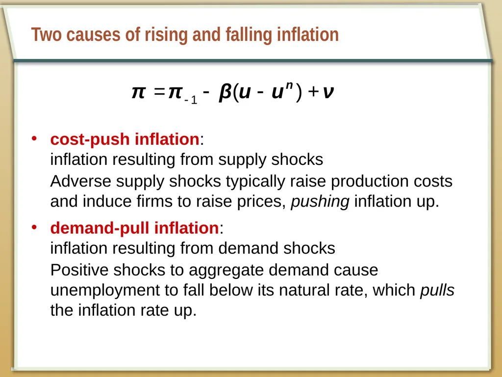
Two causes of rising and falling inflation cost-push inflation:
inflation resulting from supply shocks
Adverse supply shocks typically raise production costs and induce firms to raise prices, pushing inflation up.
demand-pull inflation: inflation resulting from demand shocks
Positive shocks to aggregate demand cause unemployment to fall below its natural rate, which pulls the inflation rate up.<br>
Adverse supply shocks typically raise production costs and induce firms to raise prices, pushing inflation up.
demand-pull inflation: inflation resulting from demand shocks
Positive shocks to aggregate demand cause unemployment to fall below its natural rate, which pulls the inflation rate up.<br>
21
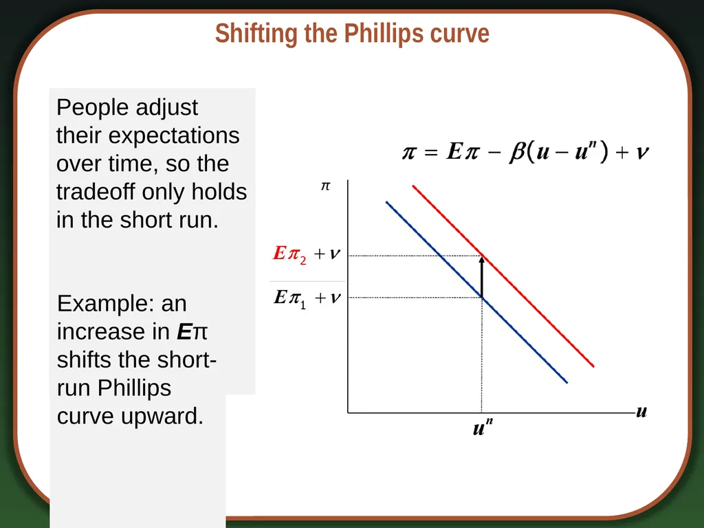
Shifting the Phillips curve People adjust their expectations over time, so the tradeoff only holds in the short run. Example: an increase in Eπ shifts the short-run Phillips curve upward.<br>
22
The sacrifice ratio, part 1 To reduce inflation, policymakers can contract aggregate demand, causing unemployment to rise above the natural rate.
The sacrifice ratio measures the percentage of a year’s real GDP that must be forgone to reduce inflation by 1 percentage point.
A typical estimate of the ratio is 5.<br>
The sacrifice ratio measures the percentage of a year’s real GDP that must be forgone to reduce inflation by 1 percentage point.
A typical estimate of the ratio is 5.<br>
23
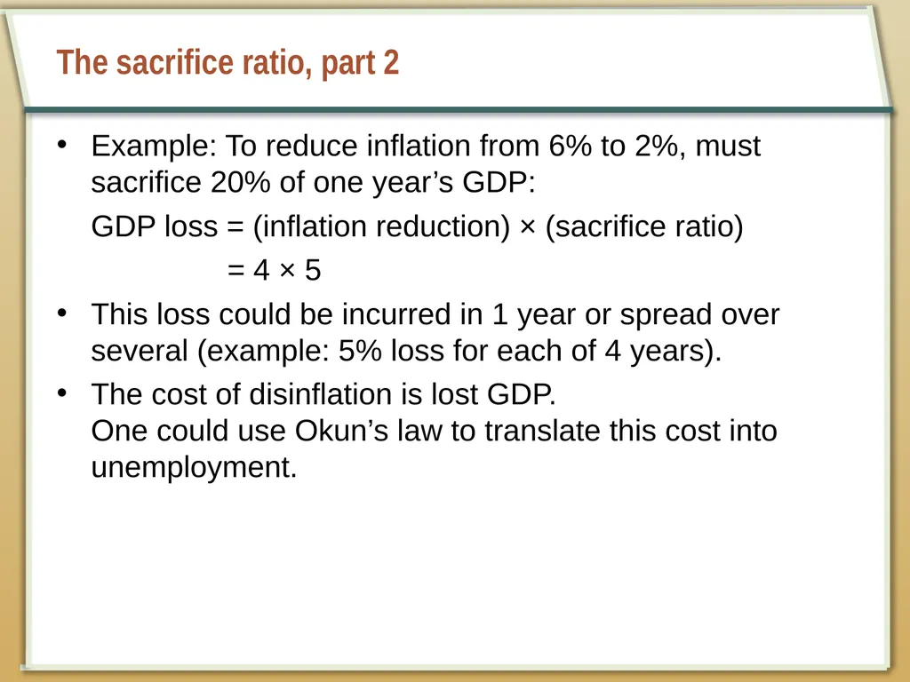
The sacrifice ratio, part 2 Example: To reduce inflation from 6% to 2%, must sacrifice 20% of one year’s GDP:
GDP loss = (inflation reduction) × (sacrifice ratio)
= 4 × 5
This loss could be incurred in 1 year or spread over several (example: 5% loss for each of 4 years).
The cost of disinflation is lost GDP. One could use Okun’s law to translate this cost into unemployment.<br>
GDP loss = (inflation reduction) × (sacrifice ratio)
= 4 × 5
This loss could be incurred in 1 year or spread over several (example: 5% loss for each of 4 years).
The cost of disinflation is lost GDP. One could use Okun’s law to translate this cost into unemployment.<br>
24
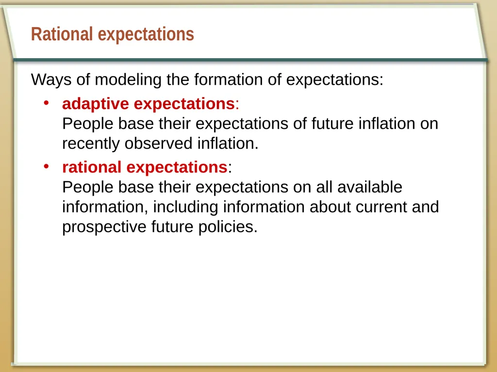
Rational expectations Ways of modeling the formation of expectations:
adaptive expectations: People base their expectations of future inflation on recently observed inflation.
rational expectations: People base their expectations on all available information, including information about current and prospective future policies.<br>
adaptive expectations: People base their expectations of future inflation on recently observed inflation.
rational expectations: People base their expectations on all available information, including information about current and prospective future policies.<br>
25
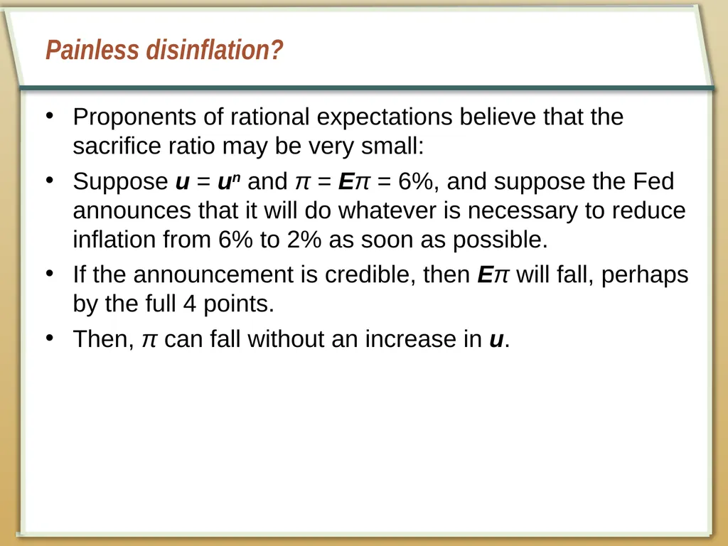
Painless disinflation? Proponents of rational expectations believe that the sacrifice ratio may be very small:
Suppose u = un and π = Eπ = 6%, and suppose the Fed announces that it will do whatever is necessary to reduce inflation from 6% to 2% as soon as possible.
If the announcement is credible, then Eπ will fall, perhaps by the full 4 points.
Then, π can fall without an increase in u.<br>
Suppose u = un and π = Eπ = 6%, and suppose the Fed announces that it will do whatever is necessary to reduce inflation from 6% to 2% as soon as possible.
If the announcement is credible, then Eπ will fall, perhaps by the full 4 points.
Then, π can fall without an increase in u.<br>
26
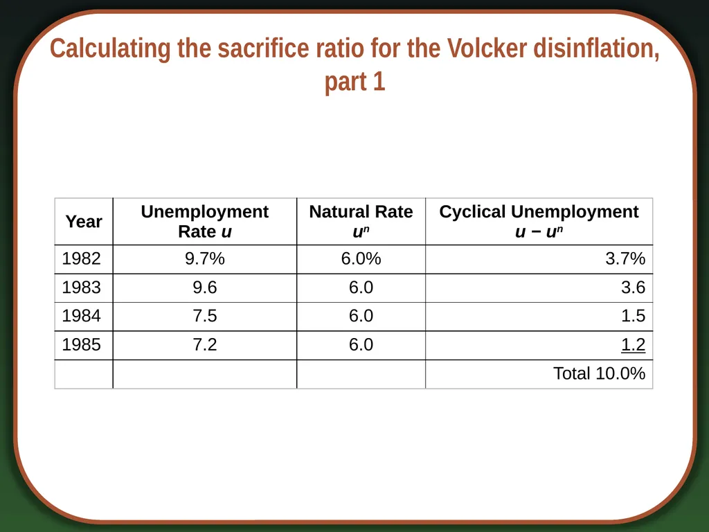
Calculating the sacrifice ratio for the Volcker disinflation, part 1<br>
27
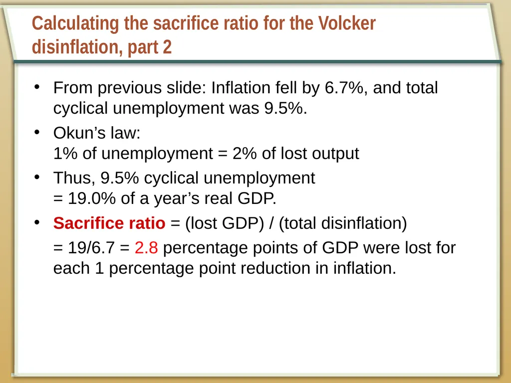
Calculating the sacrifice ratio for the Volcker disinflation, part 2 From previous slide: Inflation fell by 6.7%, and total cyclical unemployment was 9.5%.
Okun’s law: 1% of unemployment = 2% of lost output
Thus, 9.5% cyclical unemployment = 19.0% of a year’s real GDP.
Sacrifice ratio = (lost GDP) / (total disinflation)
= 19/6.7 = 2.8 percentage points of GDP were lost for each 1 percentage point reduction in inflation.<br>
Okun’s law: 1% of unemployment = 2% of lost output
Thus, 9.5% cyclical unemployment = 19.0% of a year’s real GDP.
Sacrifice ratio = (lost GDP) / (total disinflation)
= 19/6.7 = 2.8 percentage points of GDP were lost for each 1 percentage point reduction in inflation.<br>
28
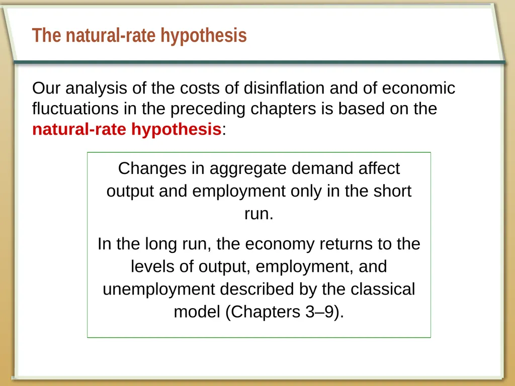
The natural-rate hypothesis Our analysis of the costs of disinflation and of economic fluctuations in the preceding chapters is based on the natural-rate hypothesis: Changes in aggregate demand affect output and employment only in the short run.
In the long run, the economy returns to the levels of output, employment, and unemployment described by the classical model (Chapters 3–9).<br>
In the long run, the economy returns to the levels of output, employment, and unemployment described by the classical model (Chapters 3–9).<br>
29
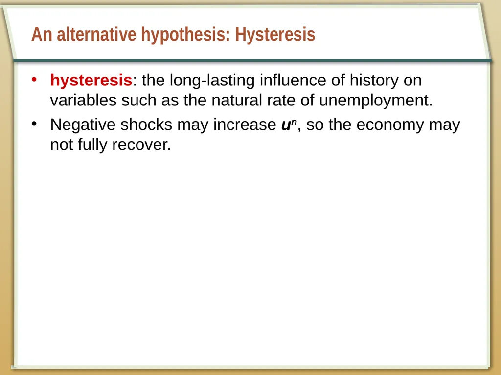
An alternative hypothesis: Hysteresis hysteresis: the long-lasting influence of history on variables such as the natural rate of unemployment.
Negative shocks may increase un, so the economy may not fully recover.<br>
Negative shocks may increase un, so the economy may not fully recover.<br>
30
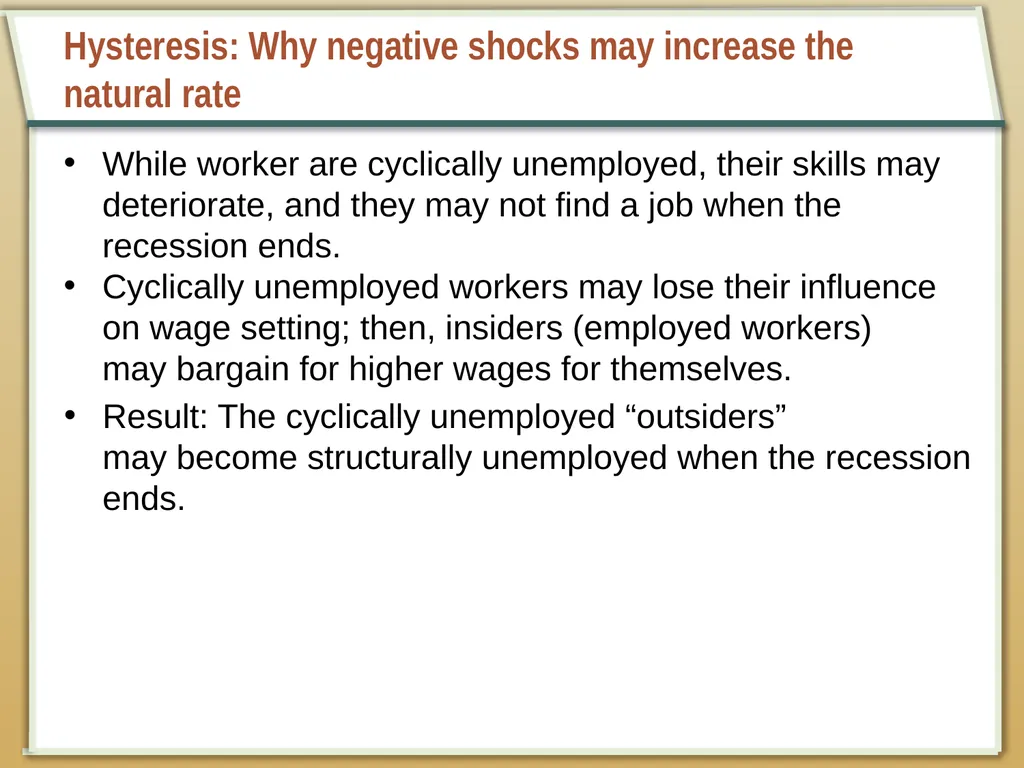
Hysteresis: Why negative shocks may increase the natural rate While worker are cyclically unemployed, their skills may deteriorate, and they may not find a job when the recession ends.
Cyclically unemployed workers may lose their influence on wage setting; then, insiders (employed workers) may bargain for higher wages for themselves.
Result: The cyclically unemployed “outsiders” may become structurally unemployed when the recession ends.<br>
Cyclically unemployed workers may lose their influence on wage setting; then, insiders (employed workers) may bargain for higher wages for themselves.
Result: The cyclically unemployed “outsiders” may become structurally unemployed when the recession ends.<br>
31
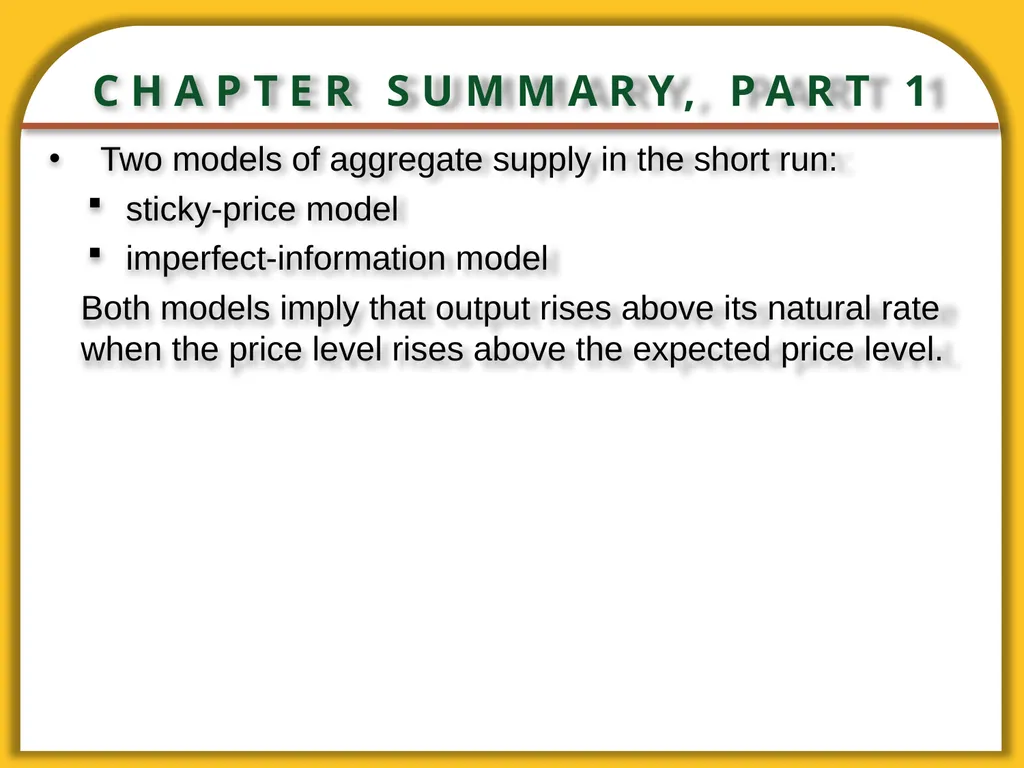
CHAPTER SUMMARY, PART 1 Two models of aggregate supply in the short run:
sticky-price model
imperfect-information model
Both models imply that output rises above its natural rate when the price level rises above the expected price level.<br>
sticky-price model
imperfect-information model
Both models imply that output rises above its natural rate when the price level rises above the expected price level.<br>
32
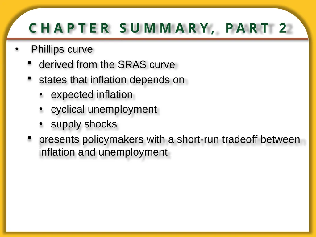
CHAPTER SUMMARY, PART 2 Phillips curve
derived from the SRAS curve
states that inflation depends on
expected inflation
cyclical unemployment
supply shocks
presents policymakers with a short-run tradeoff between inflation and unemployment<br>
derived from the SRAS curve
states that inflation depends on
expected inflation
cyclical unemployment
supply shocks
presents policymakers with a short-run tradeoff between inflation and unemployment<br>
33
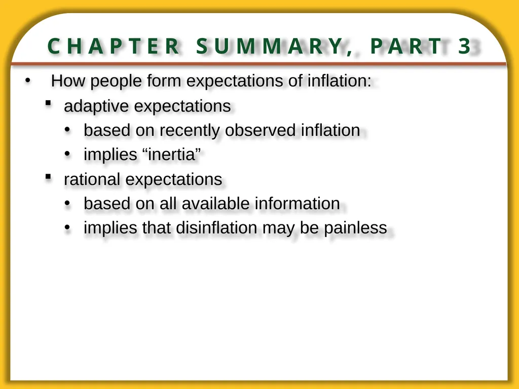
CHAPTER SUMMARY, PART 3 How people form expectations of inflation:
adaptive expectations
based on recently observed inflation
implies “inertia”
rational expectations
based on all available information
implies that disinflation may be painless<br>
adaptive expectations
based on recently observed inflation
implies “inertia”
rational expectations
based on all available information
implies that disinflation may be painless<br>
34
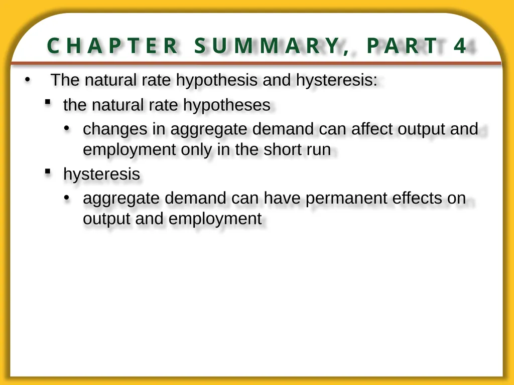
CHAPTER SUMMARY, PART 4 The natural rate hypothesis and hysteresis:
the natural rate hypotheses
changes in aggregate demand can affect output and employment only in the short run
hysteresis
aggregate demand can have permanent effects on output and employment<br>
the natural rate hypotheses
changes in aggregate demand can affect output and employment only in the short run
hysteresis
aggregate demand can have permanent effects on output and employment<br>