
Chapter 8 Decision Analysis Problem Formulation
BR
Published · 27 slides · 0 views
1 / 1
Description
Chapter 8 Decision Analysis Problem Formulation Decision Making without Probabilities Decision Making with Probabilities Risk Analysis and Sensitivity Analysis Decision Analysis with Sample Information Computing Branch Probabilities Problem
Related Topics
Share
Embed code
Download this presentation From Below
"Chapter 8 Decision Analysis Problem Formulation" is the property of its rightful owner. Permission is granted to download and print the materials on this website for personal, non-commercial use only, and to display it on your personal computer provided you do not modify the materials and that you retain all copyright notices contained in the materials. By downloading content from our website, you accept the terms of this agreement.
Presentation Transcript
01
Chapter 8
Decision Analysis Problem Formulation
Decision Making without Probabilities
Decision Making with Probabilities
Risk Analysis and Sensitivity Analysis
Decision Analysis with Sample Information
Computing Branch Probabilities<br>
Decision Making without Probabilities
Decision Making with Probabilities
Risk Analysis and Sensitivity Analysis
Decision Analysis with Sample Information
Computing Branch Probabilities<br>
02
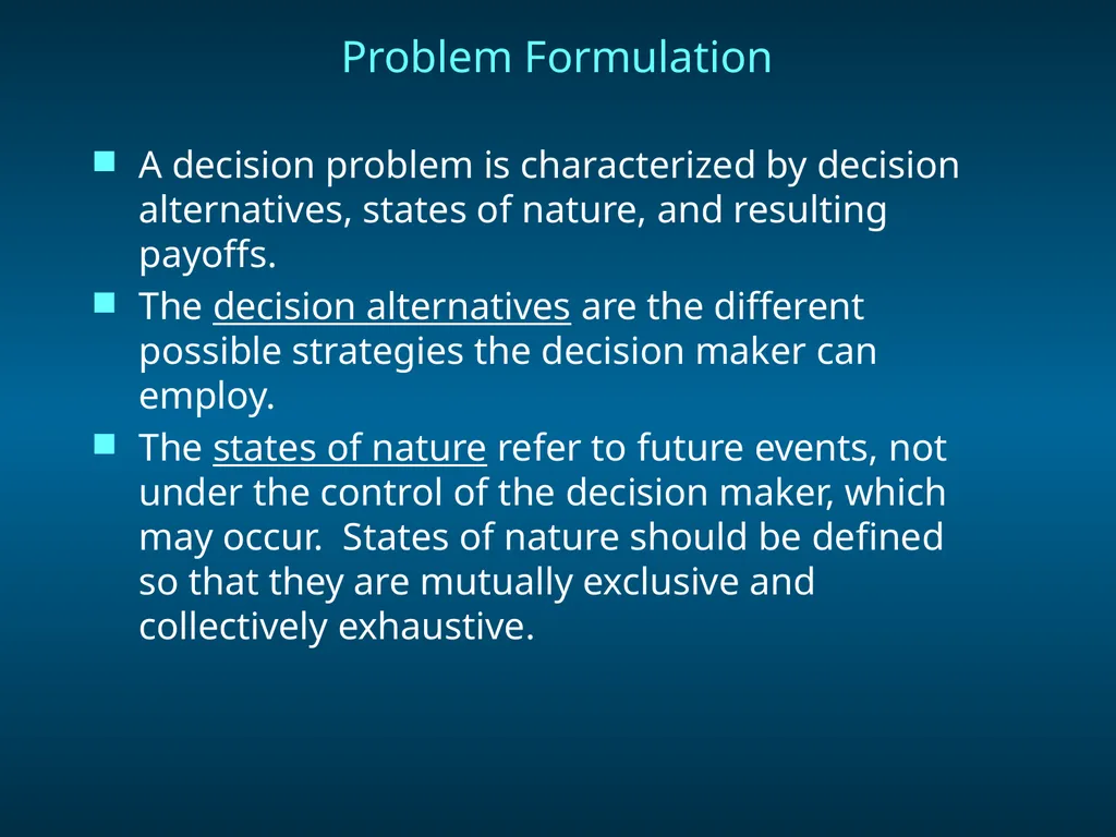
Problem Formulation A decision problem is characterized by decision alternatives, states of nature, and resulting payoffs.
The decision alternatives are the different possible strategies the decision maker can employ.
The states of nature refer to future events, not under the control of the decision maker, which may occur. States of nature should be defined so that they are mutually exclusive and collectively exhaustive.<br>
The decision alternatives are the different possible strategies the decision maker can employ.
The states of nature refer to future events, not under the control of the decision maker, which may occur. States of nature should be defined so that they are mutually exclusive and collectively exhaustive.<br>
03
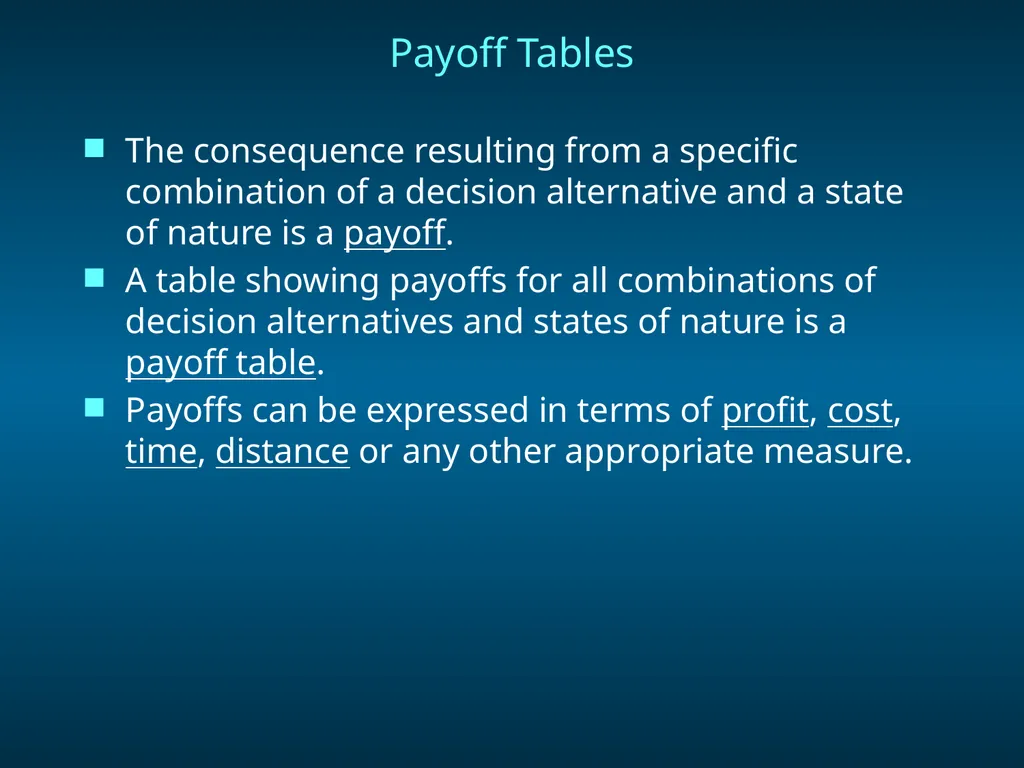
Payoff Tables The consequence resulting from a specific combination of a decision alternative and a state of nature is a payoff.
A table showing payoffs for all combinations of decision alternatives and states of nature is a payoff table.
Payoffs can be expressed in terms of profit, cost, time, distance or any other appropriate measure.<br>
A table showing payoffs for all combinations of decision alternatives and states of nature is a payoff table.
Payoffs can be expressed in terms of profit, cost, time, distance or any other appropriate measure.<br>
04
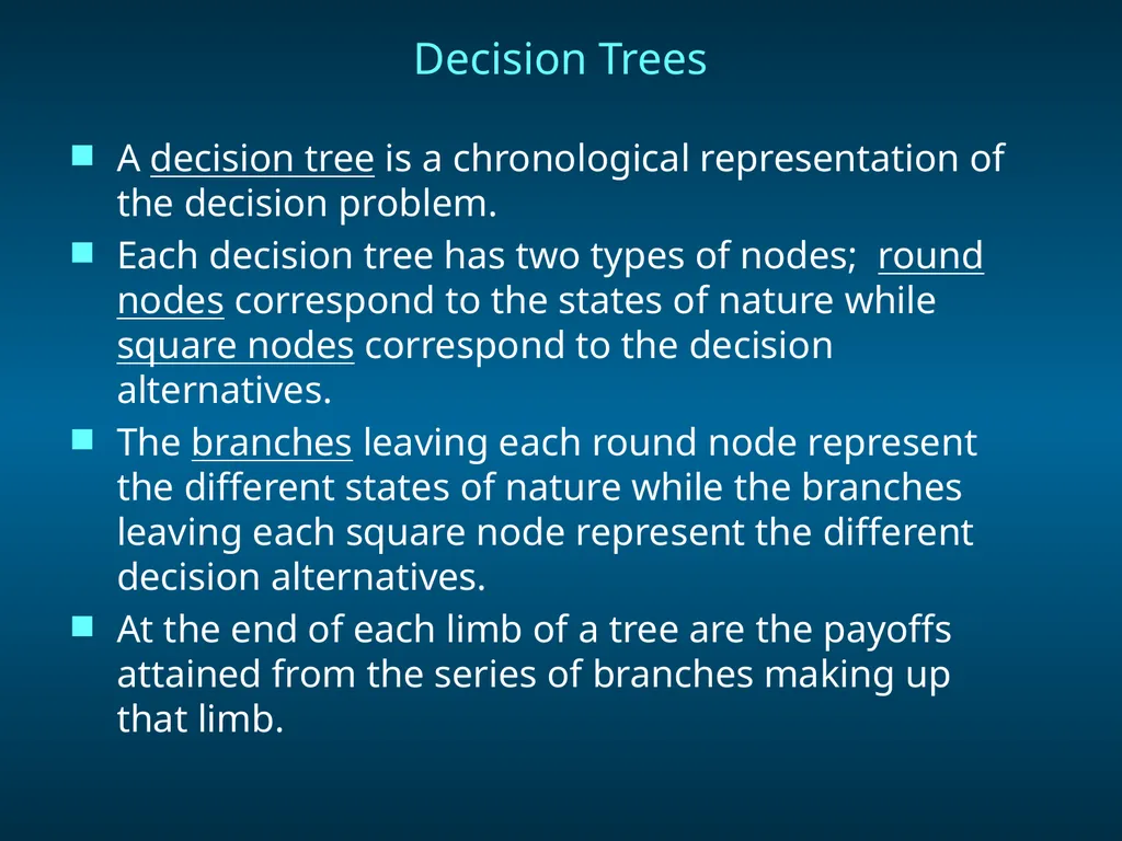
Decision Trees A decision tree is a chronological representation of the decision problem.
Each decision tree has two types of nodes; round nodes correspond to the states of nature while square nodes correspond to the decision alternatives.
The branches leaving each round node represent the different states of nature while the branches leaving each square node represent the different decision alternatives.
At the end of each limb of a tree are the payoffs attained from the series of branches making up that limb.<br>
Each decision tree has two types of nodes; round nodes correspond to the states of nature while square nodes correspond to the decision alternatives.
The branches leaving each round node represent the different states of nature while the branches leaving each square node represent the different decision alternatives.
At the end of each limb of a tree are the payoffs attained from the series of branches making up that limb.<br>
05
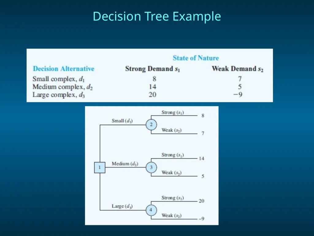
Decision Tree Example<br>
06
Decision Making without Probabilities Three commonly used criteria for decision making when probability information regarding the likelihood of the states of nature is unavailable are:
the optimistic approach
the conservative approach
the minimax regret approach.<br>
the optimistic approach
the conservative approach
the minimax regret approach.<br>
07
Optimistic Approach The optimistic approach would be used by an optimistic decision maker.
The decision with the largest possible payoff is chosen.
If the payoff table was in terms of costs, the decision with the lowest cost would be chosen.<br>
The decision with the largest possible payoff is chosen.
If the payoff table was in terms of costs, the decision with the lowest cost would be chosen.<br>
08
Conservative Approach The conservative approach would be used by a conservative decision maker.
For each decision the minimum payoff is listed and then the decision corresponding to the maximum of these minimum payoffs is selected. (Hence, the minimum possible payoff is maximized.)
If the payoff was in terms of costs, the maximum costs would be determined for each decision and then the decision corresponding to the minimum of these maximum costs is selected. (Hence, the maximum possible cost is minimized.)<br>
For each decision the minimum payoff is listed and then the decision corresponding to the maximum of these minimum payoffs is selected. (Hence, the minimum possible payoff is maximized.)
If the payoff was in terms of costs, the maximum costs would be determined for each decision and then the decision corresponding to the minimum of these maximum costs is selected. (Hence, the maximum possible cost is minimized.)<br>
09
Minimax Regret Approach The minimax regret approach requires the construction of a regret table or an opportunity loss table.
This is done by calculating for each state of nature the difference between each payoff and the largest payoff for that state of nature.
Then, using this regret table, the maximum regret for each possible decision is listed.
The decision chosen is the one corresponding to the minimum of the maximum regrets.<br>
This is done by calculating for each state of nature the difference between each payoff and the largest payoff for that state of nature.
Then, using this regret table, the maximum regret for each possible decision is listed.
The decision chosen is the one corresponding to the minimum of the maximum regrets.<br>
10
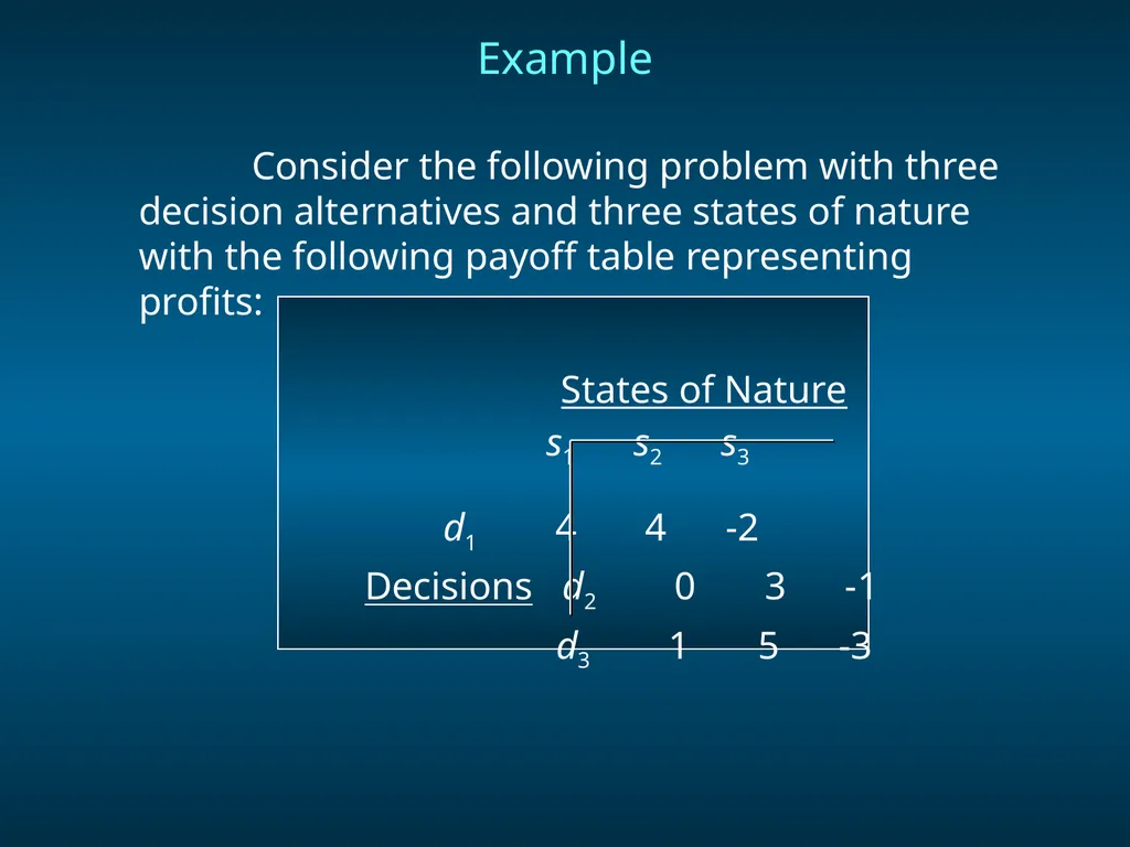
Example Consider the following problem with three decision alternatives and three states of nature with the following payoff table representing profits:
States of Nature
s1 s2 s3
d1 4 4 -2
Decisions d2 0 3 -1
d3 1 5 -3<br>
States of Nature
s1 s2 s3
d1 4 4 -2
Decisions d2 0 3 -1
d3 1 5 -3<br>
11
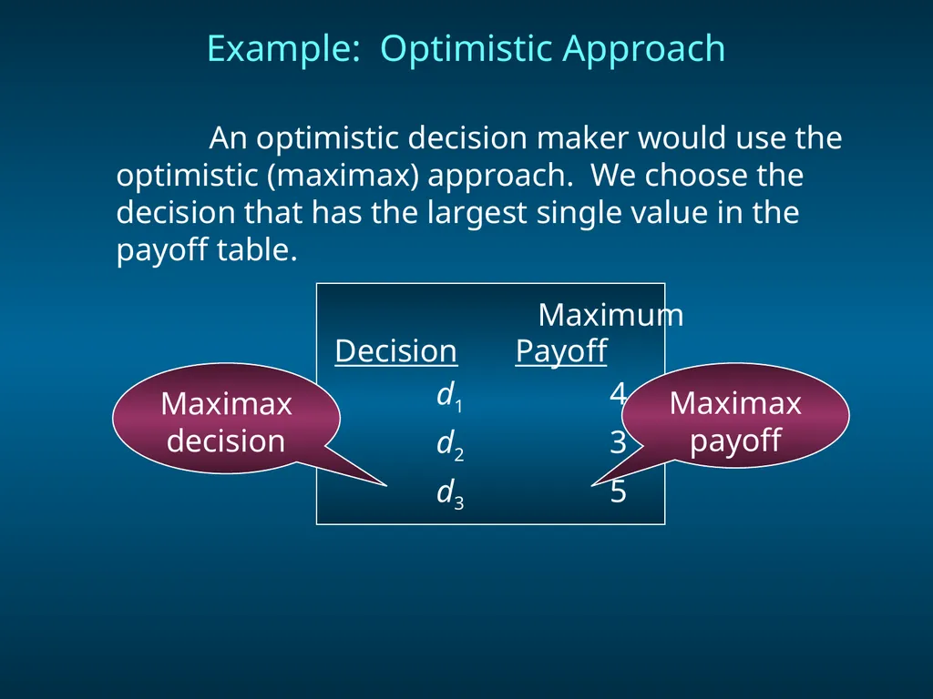
Example: Optimistic Approach An optimistic decision maker would use the optimistic (maximax) approach. We choose the decision that has the largest single value in the payoff table.
Maximum
Decision Payoff
d1 4
d2 3
d3 5 Maximax
payoff Maximaxdecision<br>
Maximum
Decision Payoff
d1 4
d2 3
d3 5 Maximax
payoff Maximaxdecision<br>
12
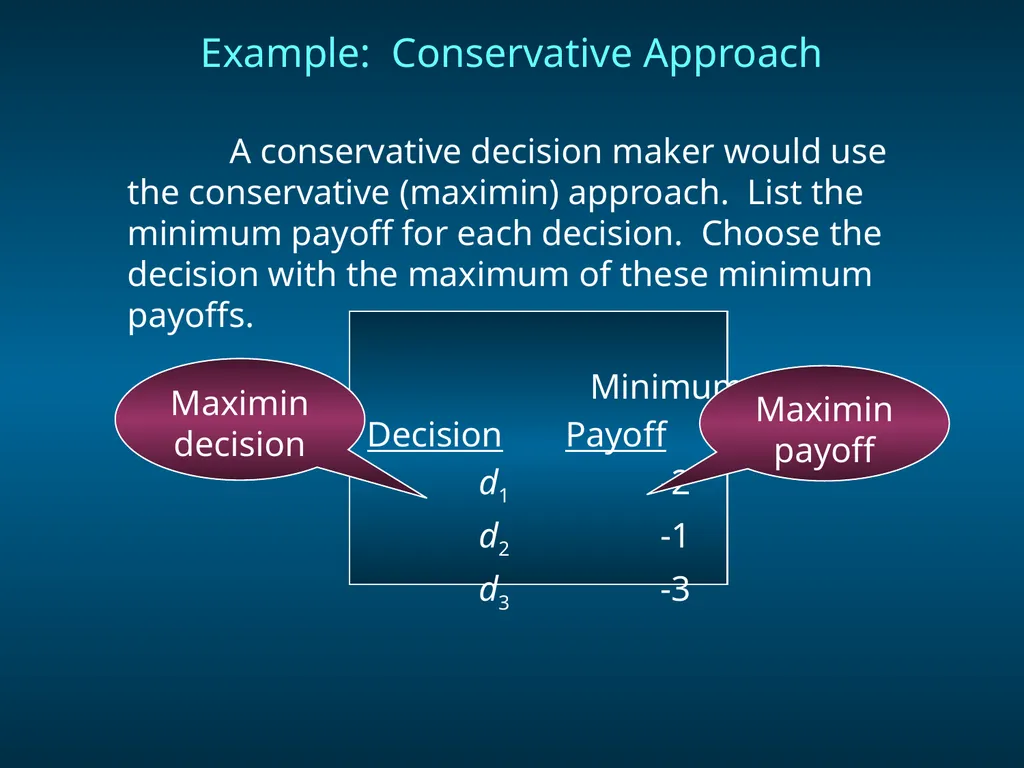
Example: Conservative Approach A conservative decision maker would use the conservative (maximin) approach. List the minimum payoff for each decision. Choose the decision with the maximum of these minimum payoffs.
Minimum
Decision Payoff
d1 -2
d2 -1
d3 -3 Maximin
decision Maximin
payoff<br>
Minimum
Decision Payoff
d1 -2
d2 -1
d3 -3 Maximin
decision Maximin
payoff<br>
13
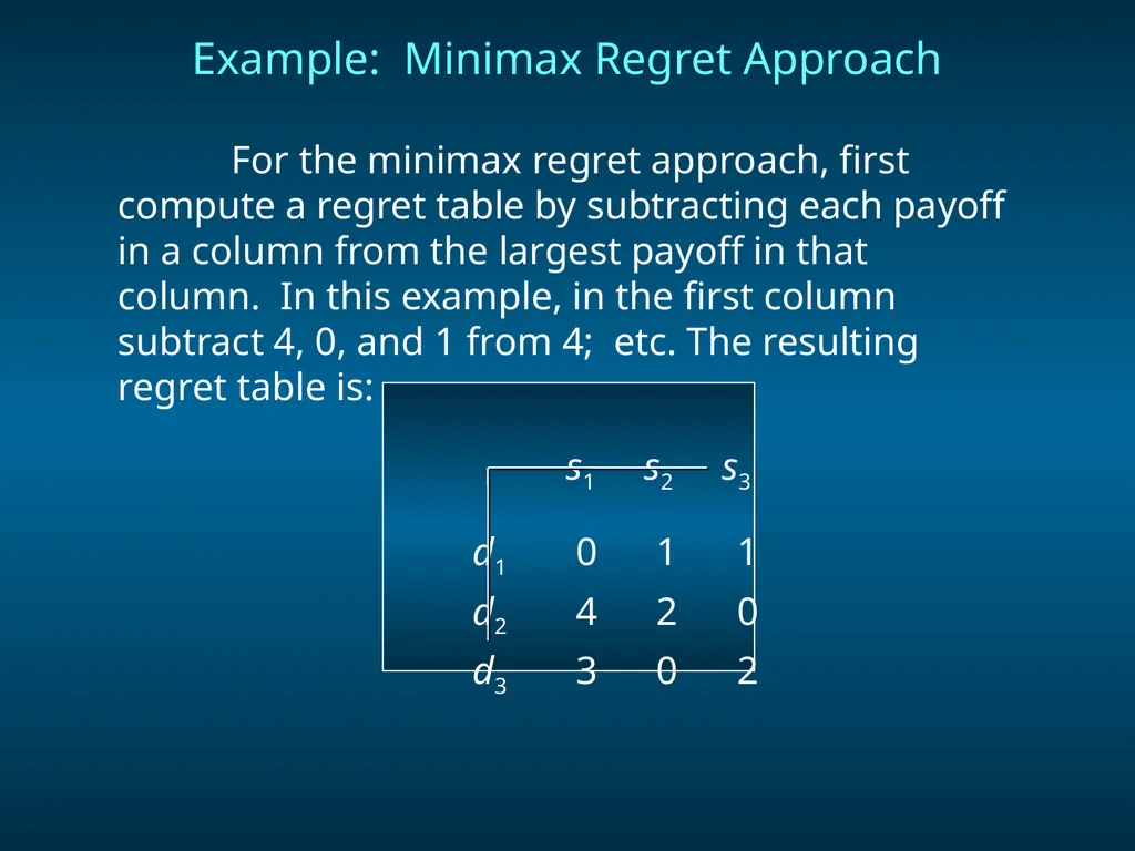
For the minimax regret approach, first compute a regret table by subtracting each payoff in a column from the largest payoff in that column. In this example, in the first column subtract 4, 0, and 1 from 4; etc. The resulting regret table is:
s1 s2 s3
d1 0 1 1
d2 4 2 0
d3 3 0 2 Example: Minimax Regret Approach<br>
s1 s2 s3
d1 0 1 1
d2 4 2 0
d3 3 0 2 Example: Minimax Regret Approach<br>
14
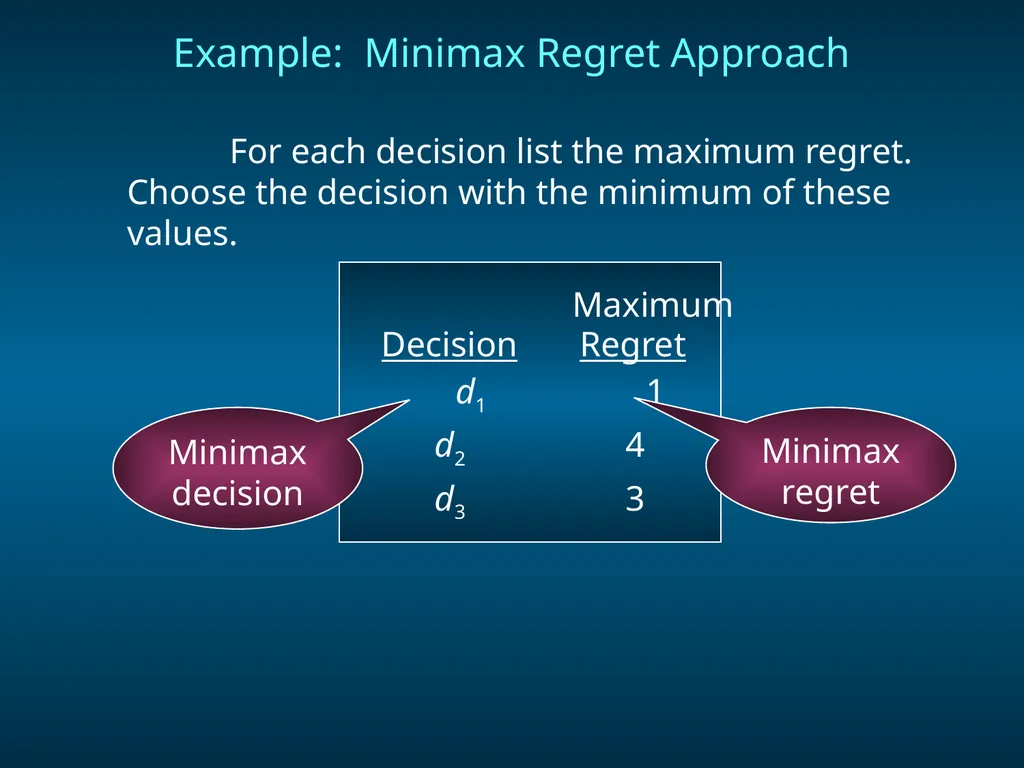
For each decision list the maximum regret. Choose the decision with the minimum of these values.
Maximum
Decision Regret
d1 1
d2 4
d3 3 Example: Minimax Regret Approach Minimax
decision Minimax
regret<br>
Maximum
Decision Regret
d1 1
d2 4
d3 3 Example: Minimax Regret Approach Minimax
decision Minimax
regret<br>
15
Decision Making with Probabilities Expected Value Approach
If probabilistic information regarding the states of nature is available, one may use the expected value (EV) approach.
Here the expected return for each decision is calculated by summing the products of the payoff under each state of nature and the probability of the respective state of nature occurring.
The decision yielding the best expected return is chosen.<br>
If probabilistic information regarding the states of nature is available, one may use the expected value (EV) approach.
Here the expected return for each decision is calculated by summing the products of the payoff under each state of nature and the probability of the respective state of nature occurring.
The decision yielding the best expected return is chosen.<br>
16
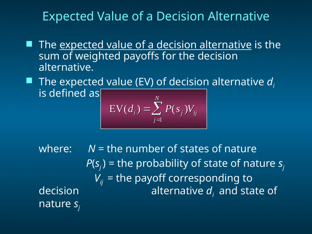
The expected value of a decision alternative is the sum of weighted payoffs for the decision alternative.
The expected value (EV) of decision alternative di is defined as:
where: N = the number of states of nature
P(sj ) = the probability of state of nature sj
Vij = the payoff corresponding to decision alternative di and state of nature sj Expected Value of a Decision Alternative<br>
The expected value (EV) of decision alternative di is defined as:
where: N = the number of states of nature
P(sj ) = the probability of state of nature sj
Vij = the payoff corresponding to decision alternative di and state of nature sj Expected Value of a Decision Alternative<br>
17
Example: Burger Prince Burger Prince Restaurant is considering opening a new restaurant on Main Street. It has three
different models, each with a different
seating capacity. Burger Prince
estimates that the average number of
customers per hour will be 80, 100, or
120. The payoff table for the three
models is on the next slide.<br>
different models, each with a different
seating capacity. Burger Prince
estimates that the average number of
customers per hour will be 80, 100, or
120. The payoff table for the three
models is on the next slide.<br>
18
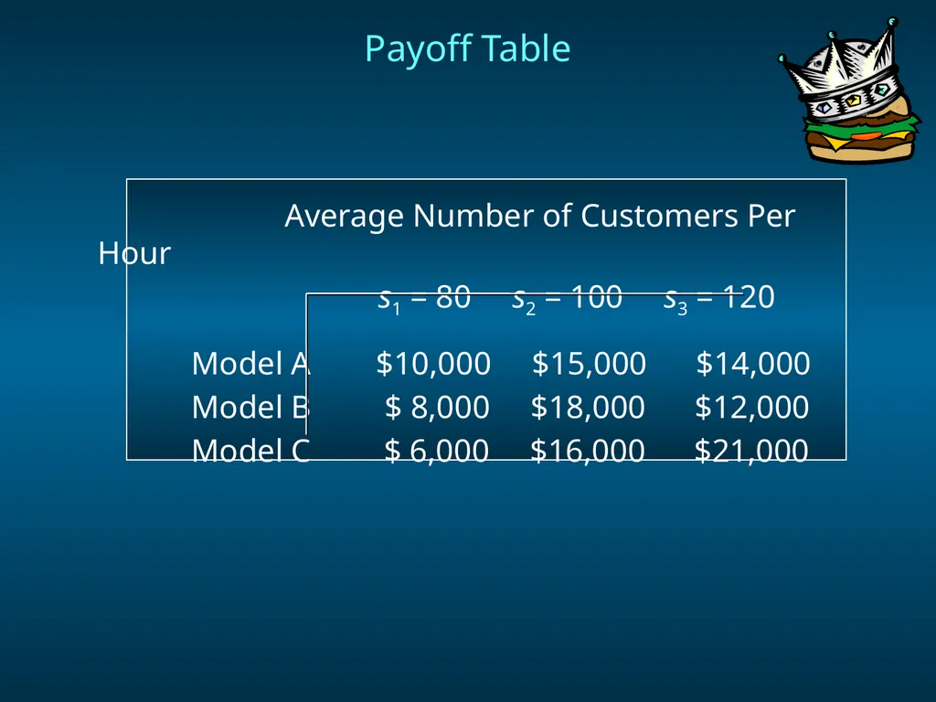
Payoff Table Average Number of Customers Per Hour
s1 = 80 s2 = 100 s3 = 120
Model A $10,000 $15,000 $14,000
Model B $ 8,000 $18,000 $12,000
Model C $ 6,000 $16,000 $21,000<br>
s1 = 80 s2 = 100 s3 = 120
Model A $10,000 $15,000 $14,000
Model B $ 8,000 $18,000 $12,000
Model C $ 6,000 $16,000 $21,000<br>
19
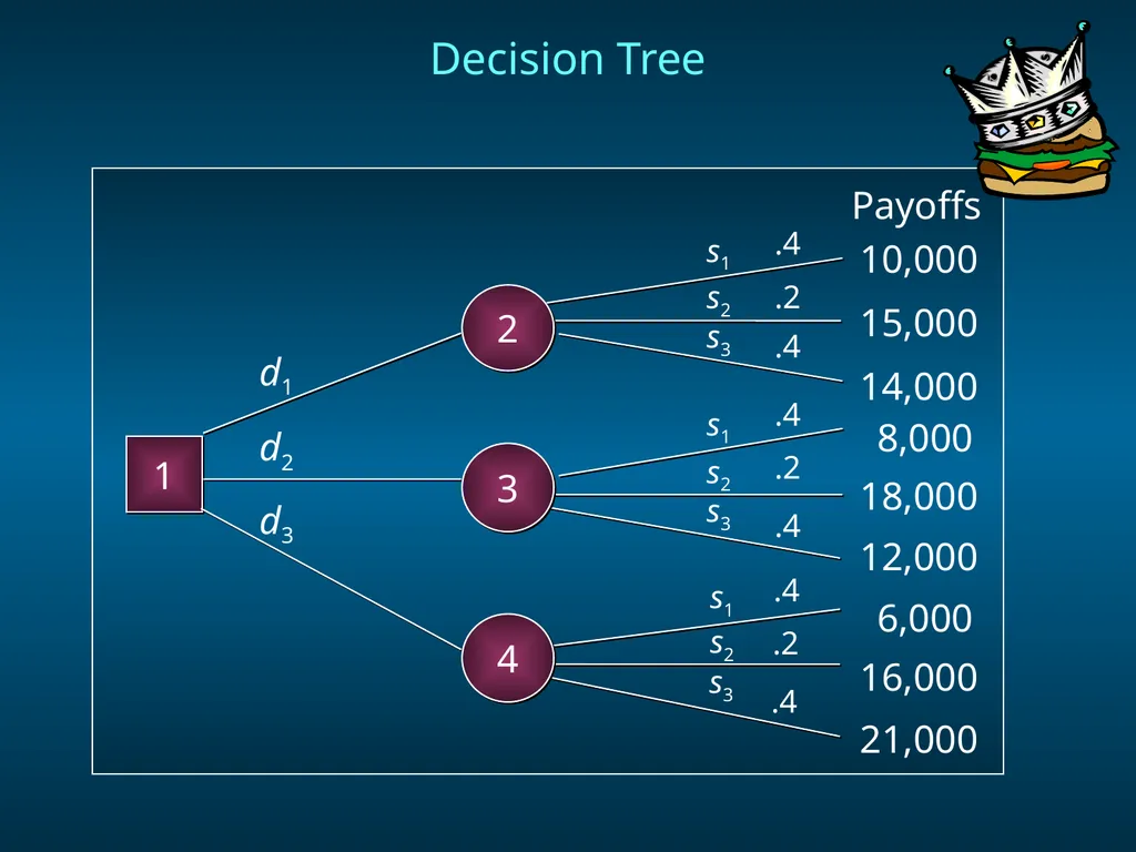
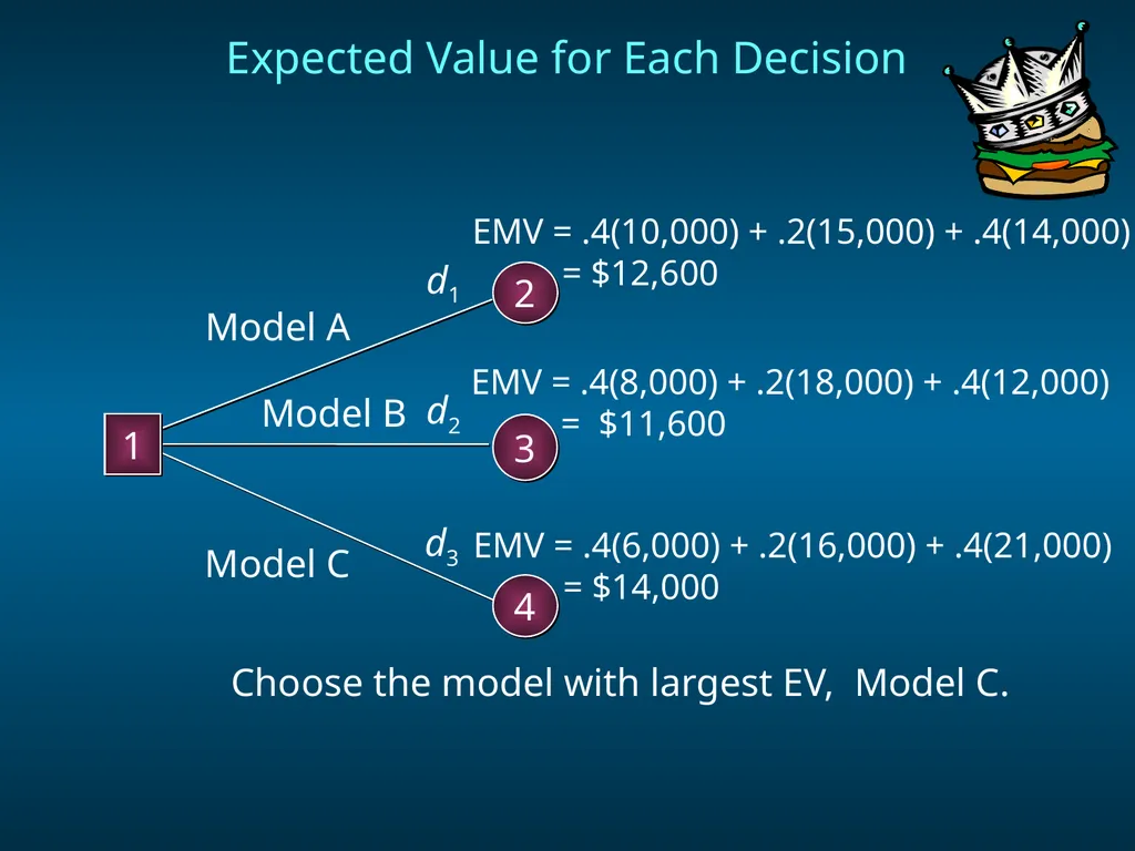
Expected Value Approach Calculate the expected value for each decision. The decision tree on the next slide can assist in this calculation. Here d1, d2, d3 represent the decision alternatives of models A, B, C, and s1, s2, s3 represent the states of nature of 80, 100, and 120.<br>
20
Decision Tree 1 .2 .4 .4 .4 .2 .4 .4 .2 .4 d1 d2 d3 s1 s1 s1 s2 s3 s2 s2 s3 s3 Payoffs 10,000 15,000 14,000 8,000 18,000 12,000 6,000 16,000 21,000 2 3 4<br>
21
Expected Value for Each Decision Choose the model with largest EV, Model C. 3 d1 d2 d3 EMV = .4(10,000) + .2(15,000) + .4(14,000)
= $12,600 EMV = .4(8,000) + .2(18,000) + .4(12,000)
= $11,600 EMV = .4(6,000) + .2(16,000) + .4(21,000)
= $14,000 Model A Model B Model C 2 1 4<br>
= $12,600 EMV = .4(8,000) + .2(18,000) + .4(12,000)
= $11,600 EMV = .4(6,000) + .2(16,000) + .4(21,000)
= $14,000 Model A Model B Model C 2 1 4<br>
22
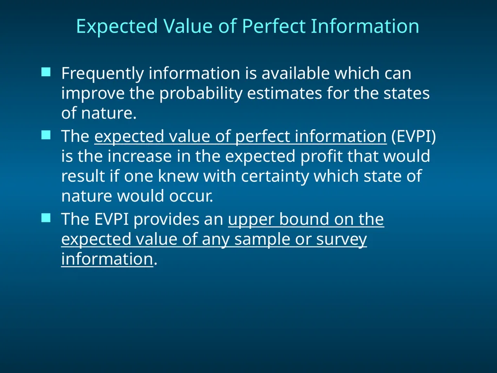
Expected Value of Perfect Information Frequently information is available which can improve the probability estimates for the states of nature.
The expected value of perfect information (EVPI) is the increase in the expected profit that would result if one knew with certainty which state of nature would occur.
The EVPI provides an upper bound on the expected value of any sample or survey information.<br>
The expected value of perfect information (EVPI) is the increase in the expected profit that would result if one knew with certainty which state of nature would occur.
The EVPI provides an upper bound on the expected value of any sample or survey information.<br>
23
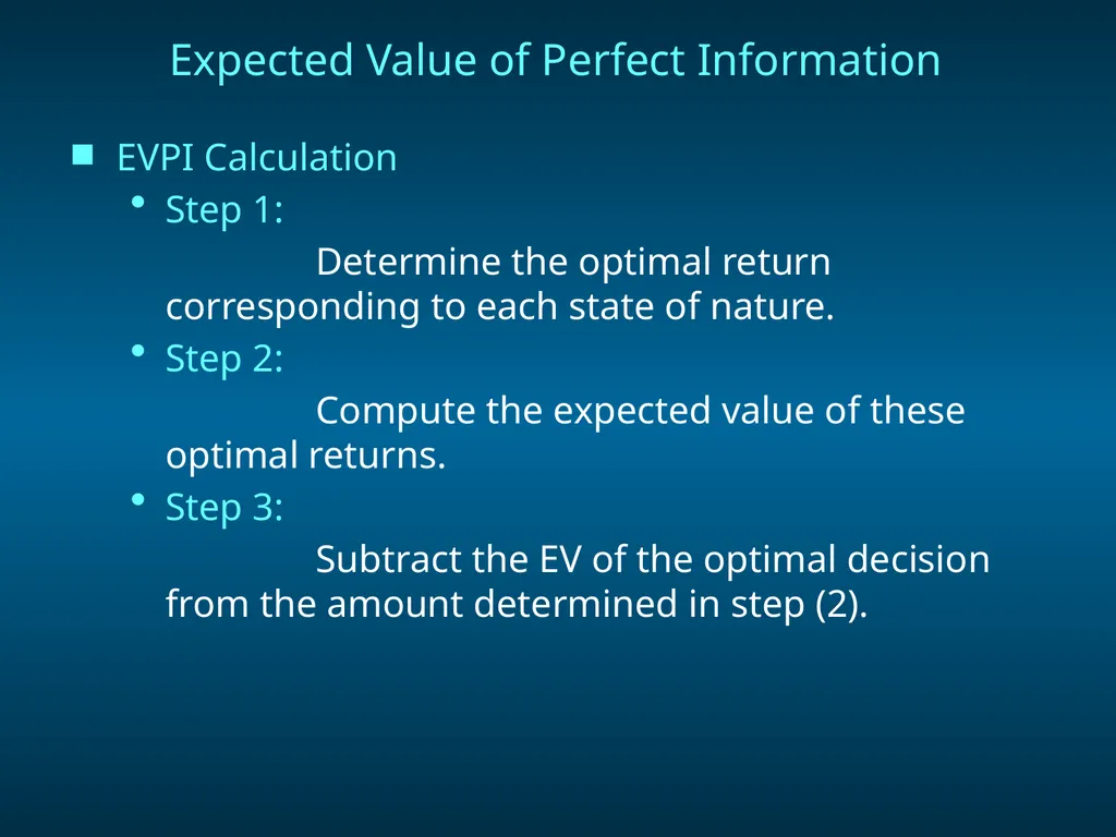
Expected Value of Perfect Information EVPI Calculation
Step 1:
Determine the optimal return corresponding to each state of nature.
Step 2:
Compute the expected value of these optimal returns.
Step 3:
Subtract the EV of the optimal decision from the amount determined in step (2).<br>
Step 1:
Determine the optimal return corresponding to each state of nature.
Step 2:
Compute the expected value of these optimal returns.
Step 3:
Subtract the EV of the optimal decision from the amount determined in step (2).<br>
24
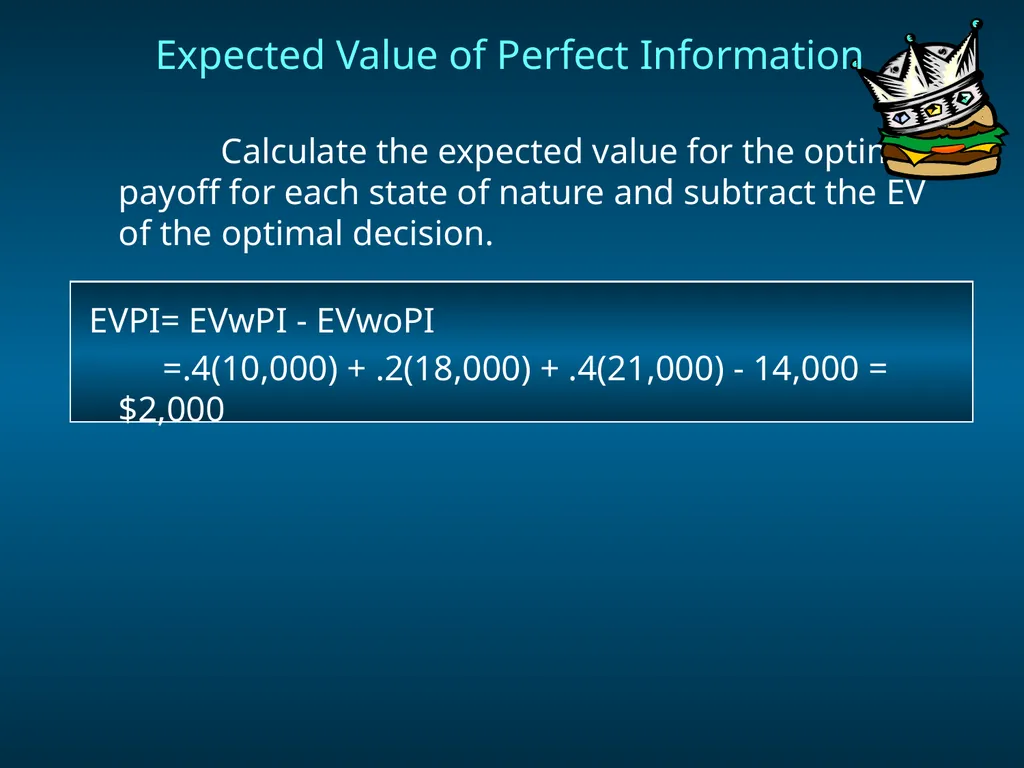
Calculate the expected value for the optimum payoff for each state of nature and subtract the EV of the optimal decision.
EVPI= EVwPI - EVwoPI
=.4(10,000) + .2(18,000) + .4(21,000) - 14,000 = $2,000 Expected Value of Perfect Information<br>
EVPI= EVwPI - EVwoPI
=.4(10,000) + .2(18,000) + .4(21,000) - 14,000 = $2,000 Expected Value of Perfect Information<br>
25
Risk Analysis Risk analysis helps the decision maker recognize the difference between:
the expected value of a decision alternative, and
the payoff that might actually occur
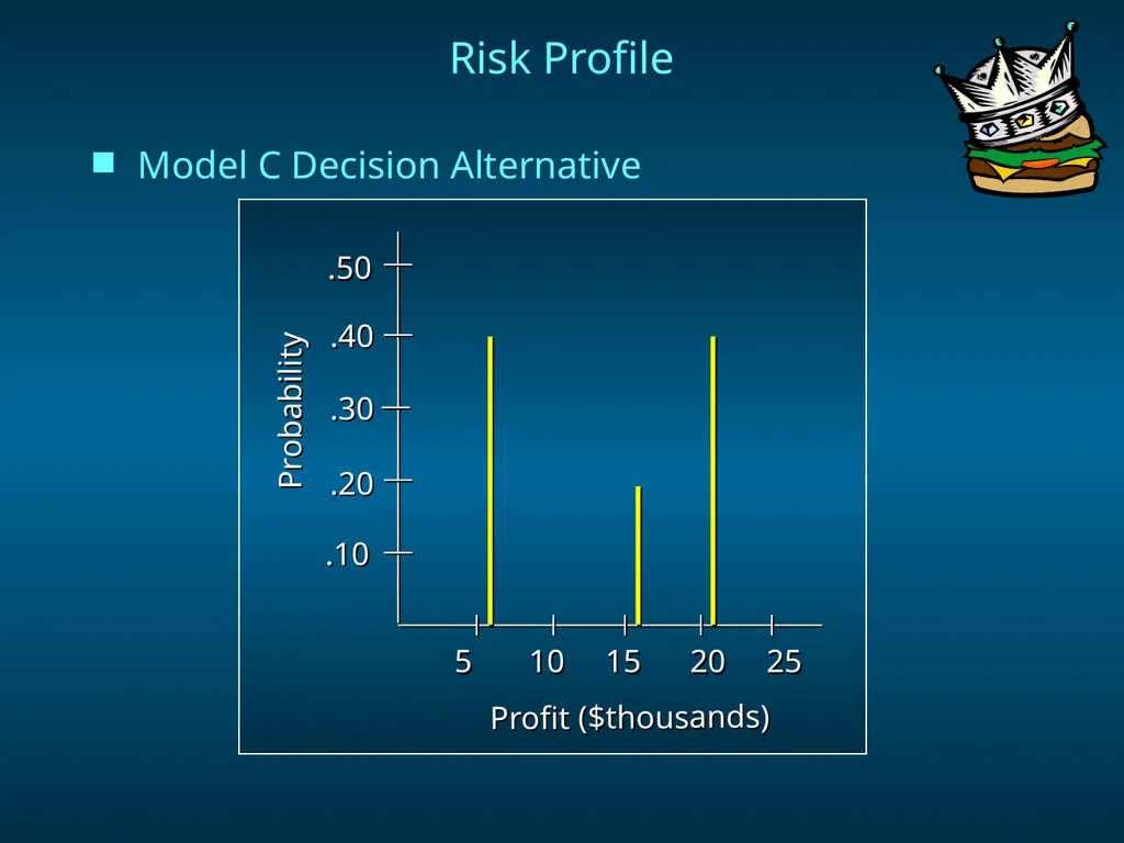
The risk profile for a decision alternative shows the possible payoffs for the decision alternative along with their associated probabilities.<br>
the expected value of a decision alternative, and
the payoff that might actually occur
The risk profile for a decision alternative shows the possible payoffs for the decision alternative along with their associated probabilities.<br>
26
Risk Profile Model C Decision Alternative .10 .20 .30 .40 .50 5 10 15 20 25 Probability Profit ($thousands)<br>
27
Sensitivity Analysis Sensitivity analysis can be used to determine how changes to the following inputs affect the recommended decision alternative:
probabilities for the states of nature
values of the payoffs
If a small change in the value of one of the inputs causes a change in the recommended decision alternative, extra effort and care should be taken in estimating the input value.<br>
probabilities for the states of nature
values of the payoffs
If a small change in the value of one of the inputs causes a change in the recommended decision alternative, extra effort and care should be taken in estimating the input value.<br>