
CPSC 531: System Modeling and Simulation Carey
Description: CPSC 531: System Modeling and Simulation Carey Williamson Department of Computer Science University of Calgary Fall 2017 The world a model-builder sees is probabilistic rather than deterministic: Some probability model might well describe
Related Topics
Download Presentation
"CPSC 531: System Modeling and Simulation Carey" is the property of its rightful owner. Permission is granted to download and print the materials on this website for personal, non-commercial use only, and to display it on your personal computer provided you do not modify the materials and that you retain all copyright notices contained in the materials. By downloading content from our website, you accept the terms of this agreement.
Presentation Transcript
slide1. CPSC 531:
System Modeling and Simulation Carey Williamson
Department of Computer Science
University of Calgary
Fall 2017<br>
slide2. The world a model-builder sees is probabilistic rather than deterministic:
Some probability model might well describe the variations
Goals:
Review the fundamental concepts of probability
Understand the difference between discrete and continuous random variable
Review the most common probability models Overview 2<br>
slide3. Probability and random variables
Random experiment and random variable
Probability mass/density functions
Expectation, variance, covariance, correlation
Probability distributions
Discrete probability distributions
Continuous probability distributions
Empirical probability distributions Outline 3<br>
slide4. Probability and random variables
Random experiment and random variable
Probability mass/density functions
Expectation, variance, covariance, correlation
Probability distributions
Discrete probability distributions
Continuous probability distributions
Empirical probability distribution Outline 4<br>
slide5. Probability 5<br>
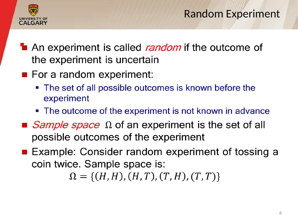
slide6. Random Experiment 6<br>
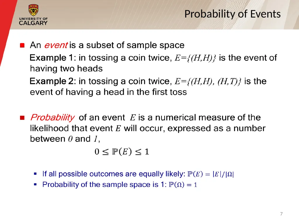
slide7. Probability of Events 7<br>
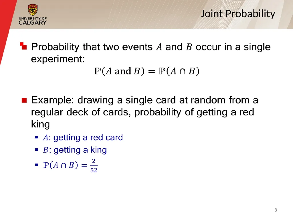
slide8. Joint Probability 8<br>
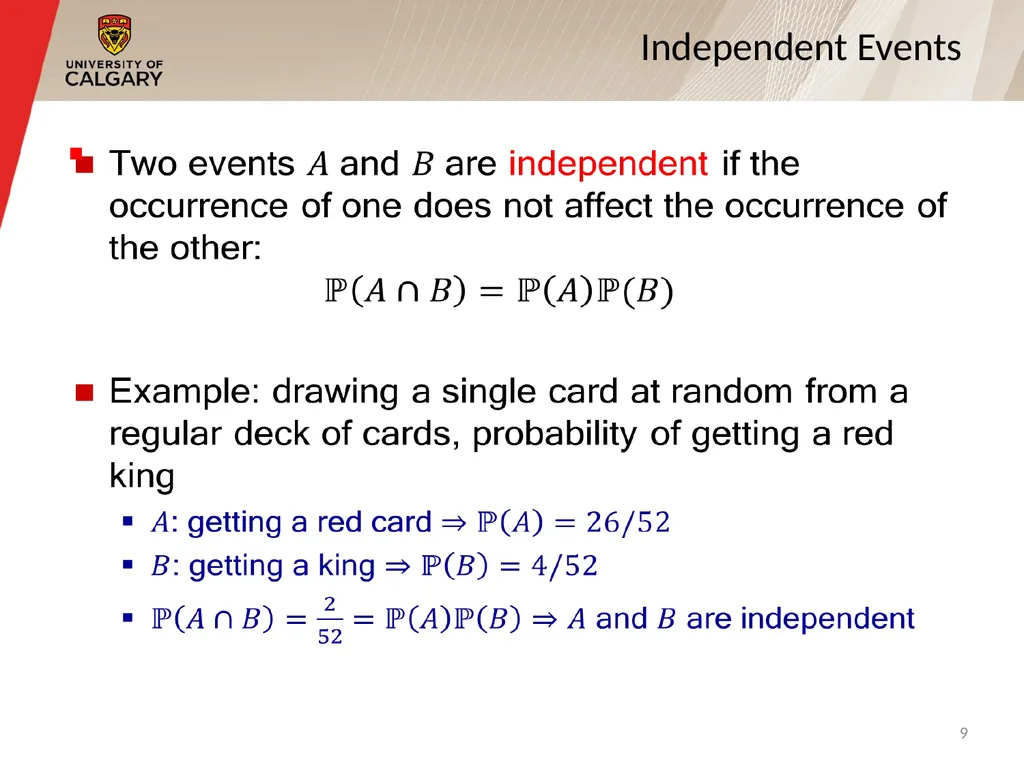
slide9. Independent Events 9<br>
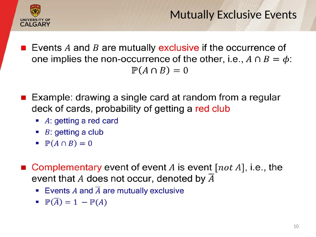
slide10. Mutually Exclusive Events 10<br>
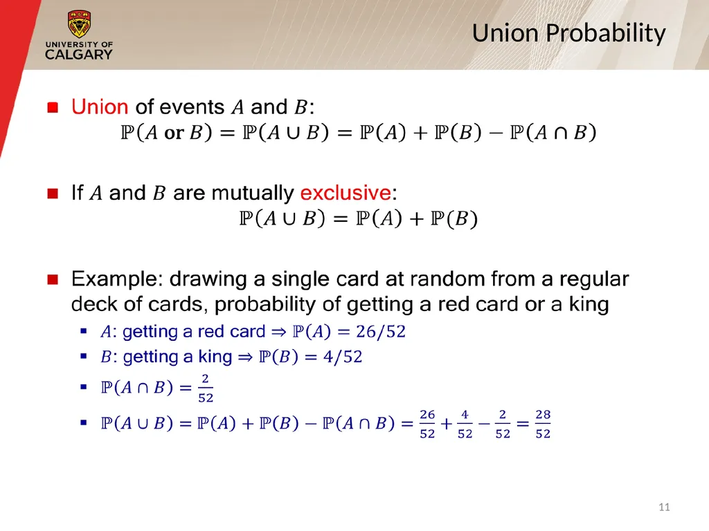
slide11. Union Probability 11<br>
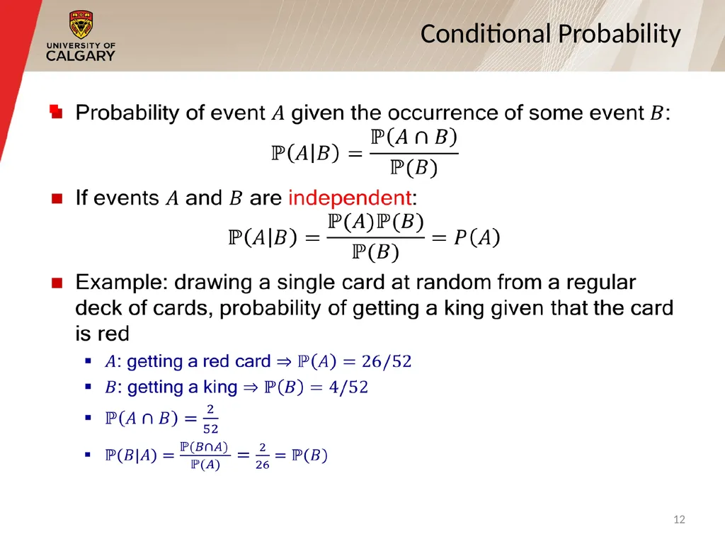
slide12. Conditional Probability 12<br>
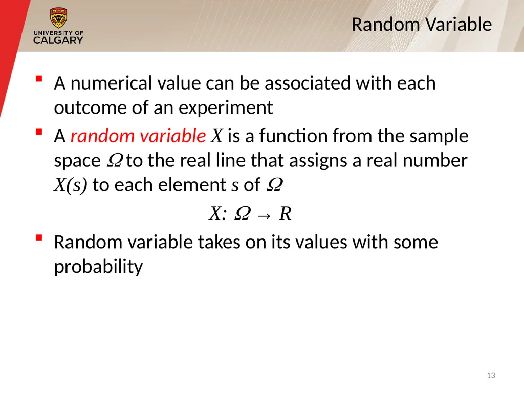
slide13. A numerical value can be associated with each outcome of an experiment
A random variable X is a function from the sample space to the real line that assigns a real number X(s) to each element s of
X: → R
Random variable takes on its values with some probability Random Variable 13<br>
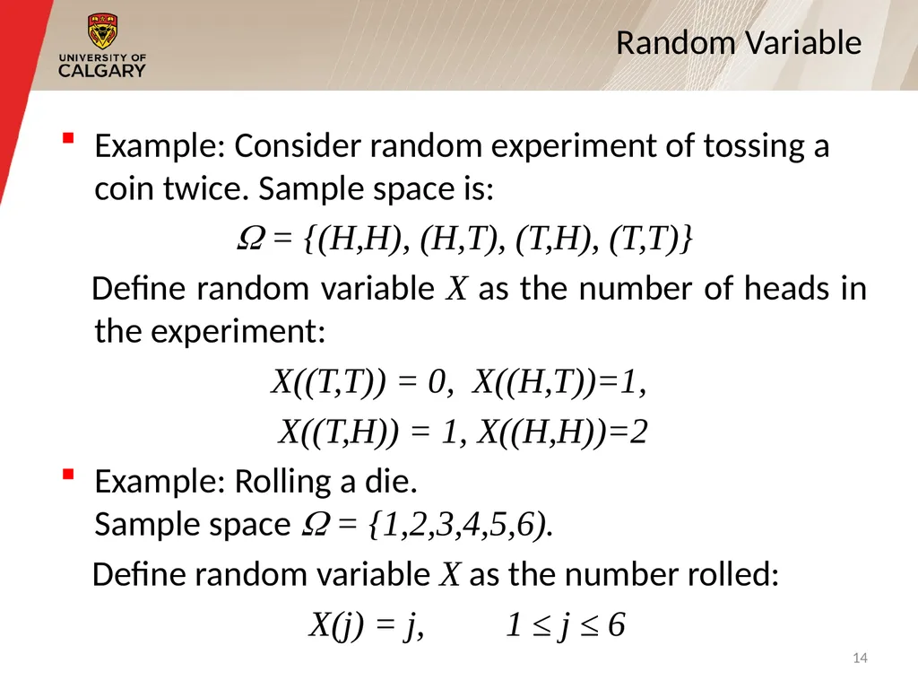
slide14. Example: Consider random experiment of tossing a coin twice. Sample space is:
= {(H,H), (H,T), (T,H), (T,T)}
Define random variable X as the number of heads in the experiment:
X((T,T)) = 0, X((H,T))=1,
X((T,H)) = 1, X((H,H))=2
Example: Rolling a die. Sample space = {1,2,3,4,5,6).
Define random variable X as the number rolled:
X(j) = j, 1 ≤ j ≤ 6 Random Variable 14<br>
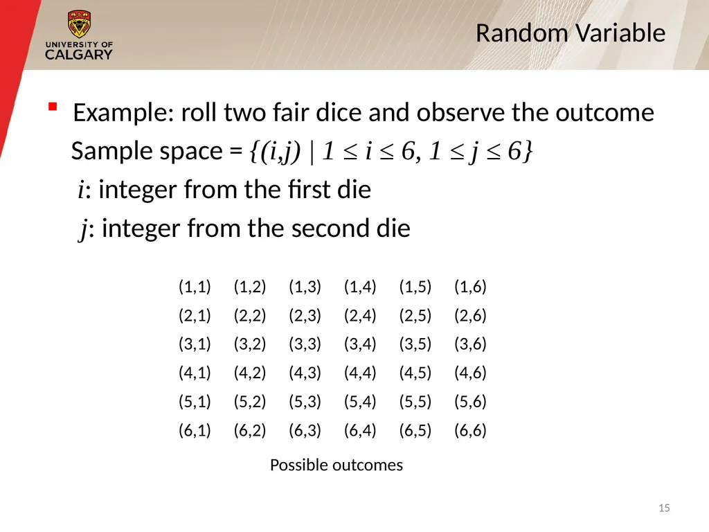
slide15. Example: roll two fair dice and observe the outcome
Sample space = {(i,j) | 1 ≤ i ≤ 6, 1 ≤ j ≤ 6}
i: integer from the first die
j: integer from the second die Random Variable Possible outcomes 15<br>
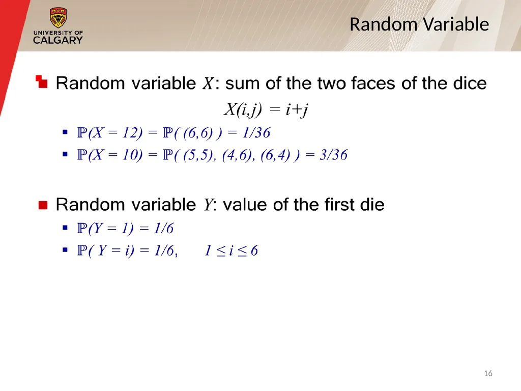
slide16. Random Variable 16<br>
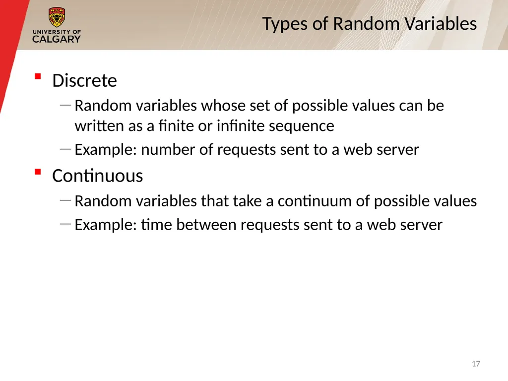
slide17. Discrete
Random variables whose set of possible values can be written as a finite or infinite sequence
Example: number of requests sent to a web server
Continuous
Random variables that take a continuum of possible values
Example: time between requests sent to a web server Types of Random Variables 17<br>
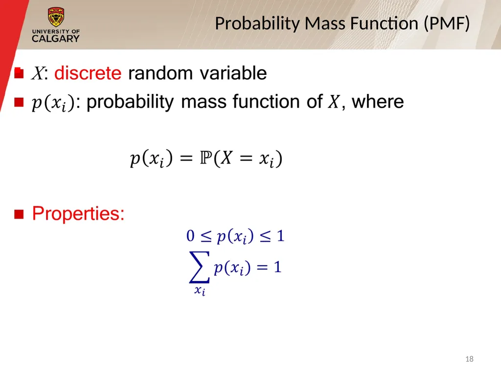
slide18. Probability Mass Function (PMF) 18<br>
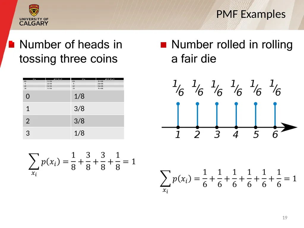
slide19. PMF Examples 19<br>
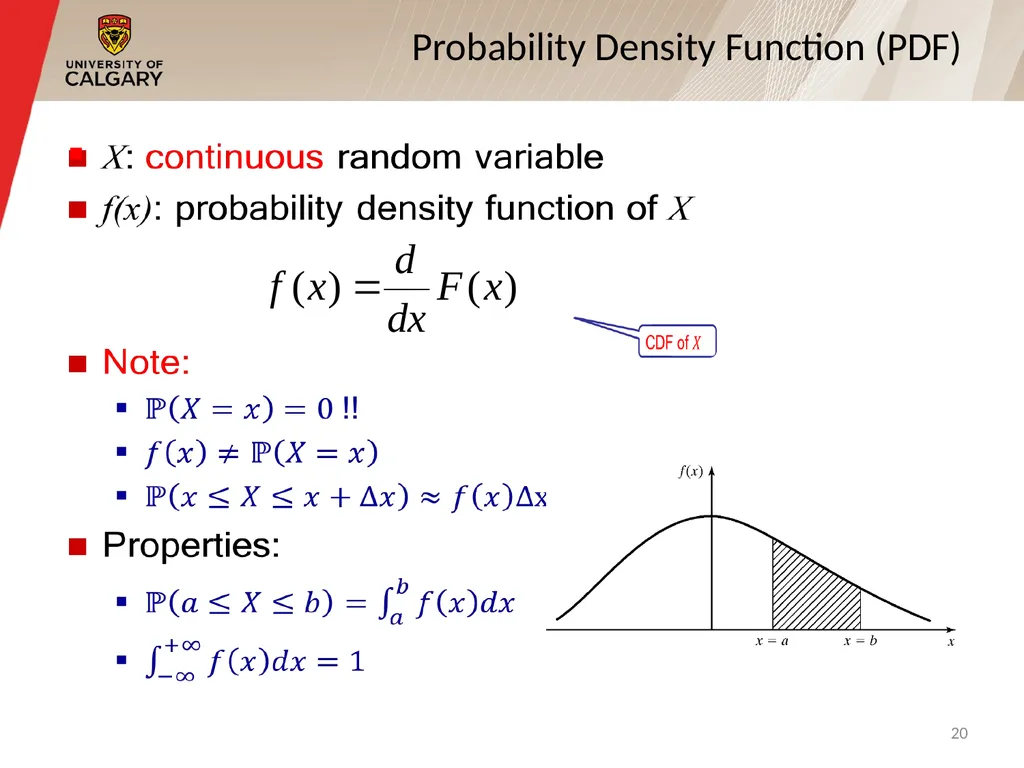
slide20. Probability Density Function (PDF) 20<br>
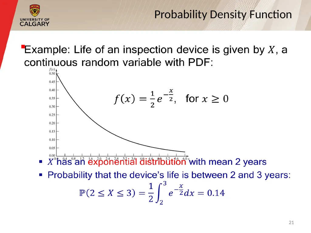
slide21. Probability Density Function 21<br>
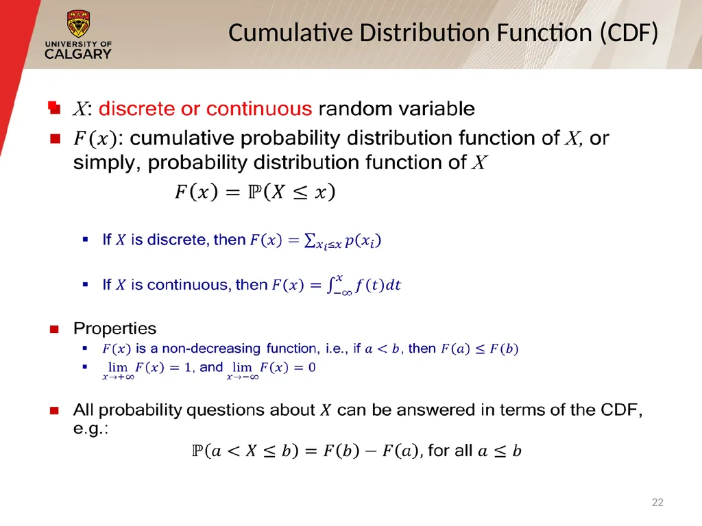
slide22. Cumulative Distribution Function (CDF) 22<br>
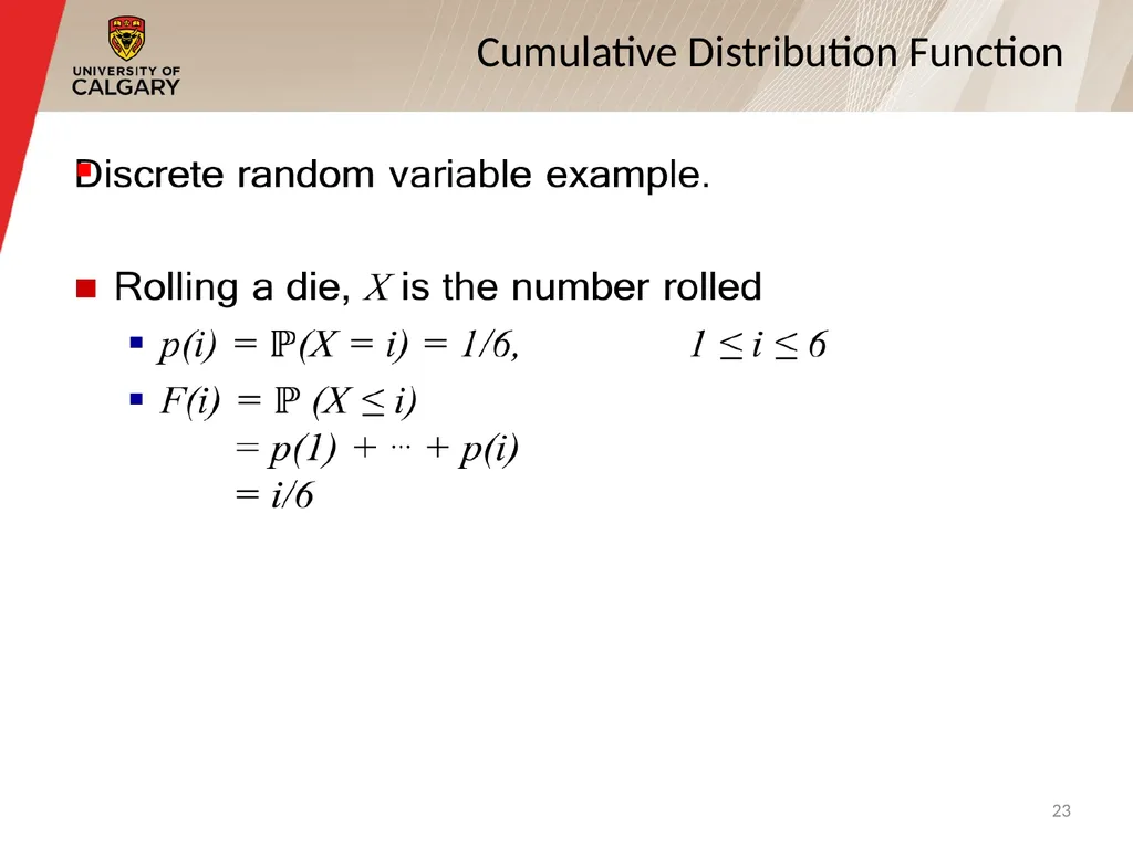
slide23. Cumulative Distribution Function 23<br>
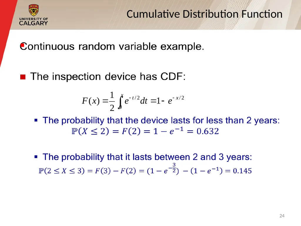
slide24. Cumulative Distribution Function 24<br>
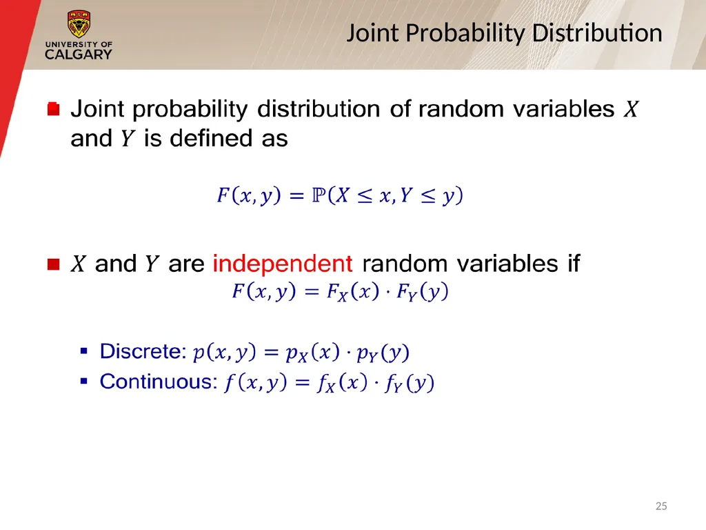
slide25. Joint Probability Distribution 25<br>
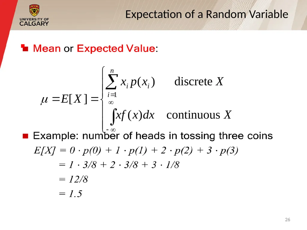
slide26. Expectation of a Random Variable 26<br>
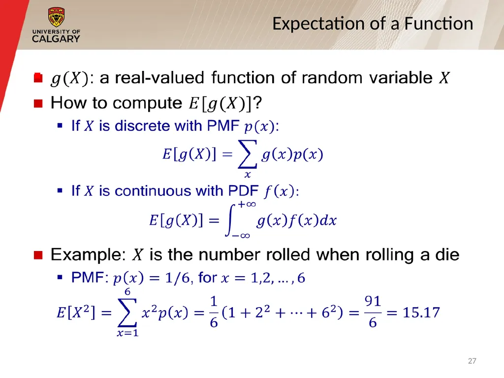
slide27. Expectation of a Function 27<br>
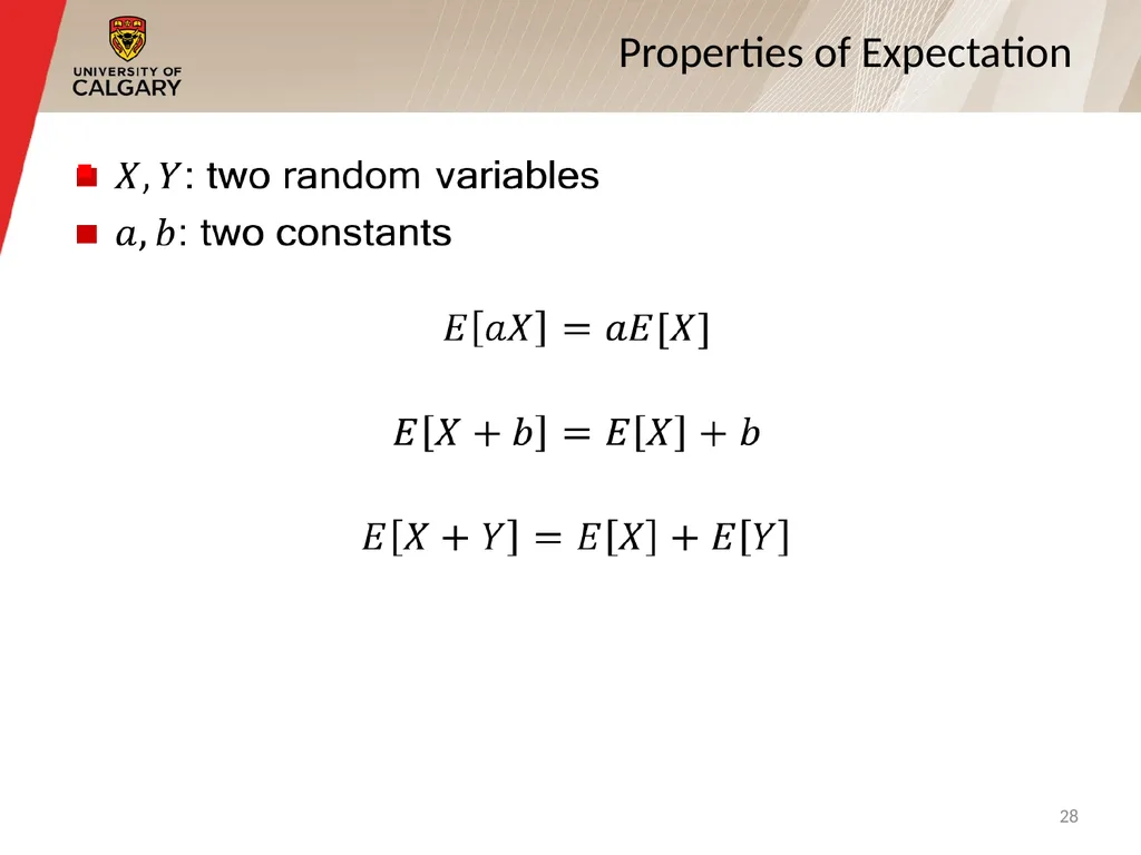
slide28. Properties of Expectation 28<br>
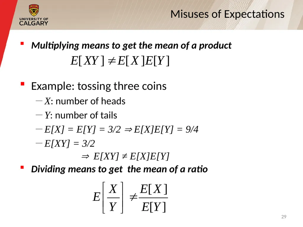
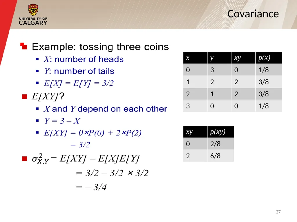
slide29. Multiplying means to get the mean of a product
Example: tossing three coins
X: number of heads
Y: number of tails
E[X] = E[Y] = 3/2 E[X]E[Y] = 9/4
E[XY] = 3/2
E[XY] ≠ E[X]E[Y]
Dividing means to get the mean of a ratio Misuses of Expectations 29<br>
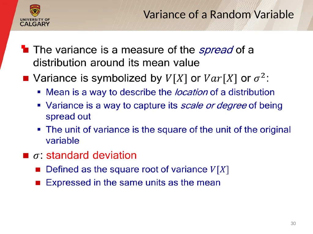
slide30. Variance of a Random Variable 30<br>
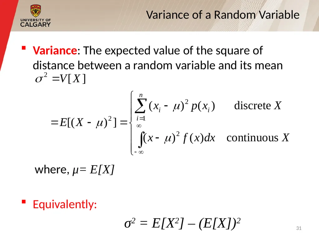
slide31. Variance: The expected value of the square of distance between a random variable and its mean
where, μ= E[X]
Equivalently:
σ2 = E[X2] – (E[X])2 Variance of a Random Variable 31<br>
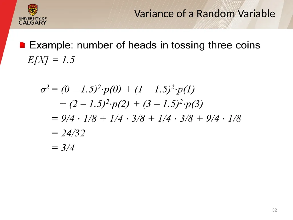
slide32. Variance of a Random Variable 32<br>
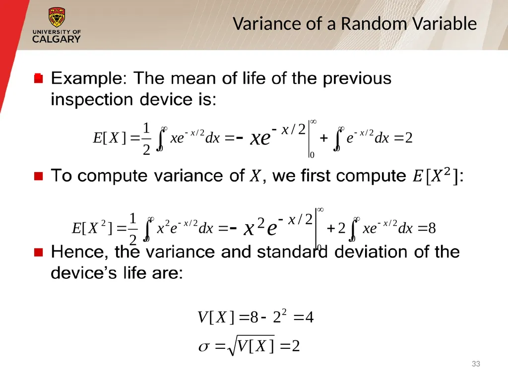
slide33. Variance of a Random Variable 33<br>
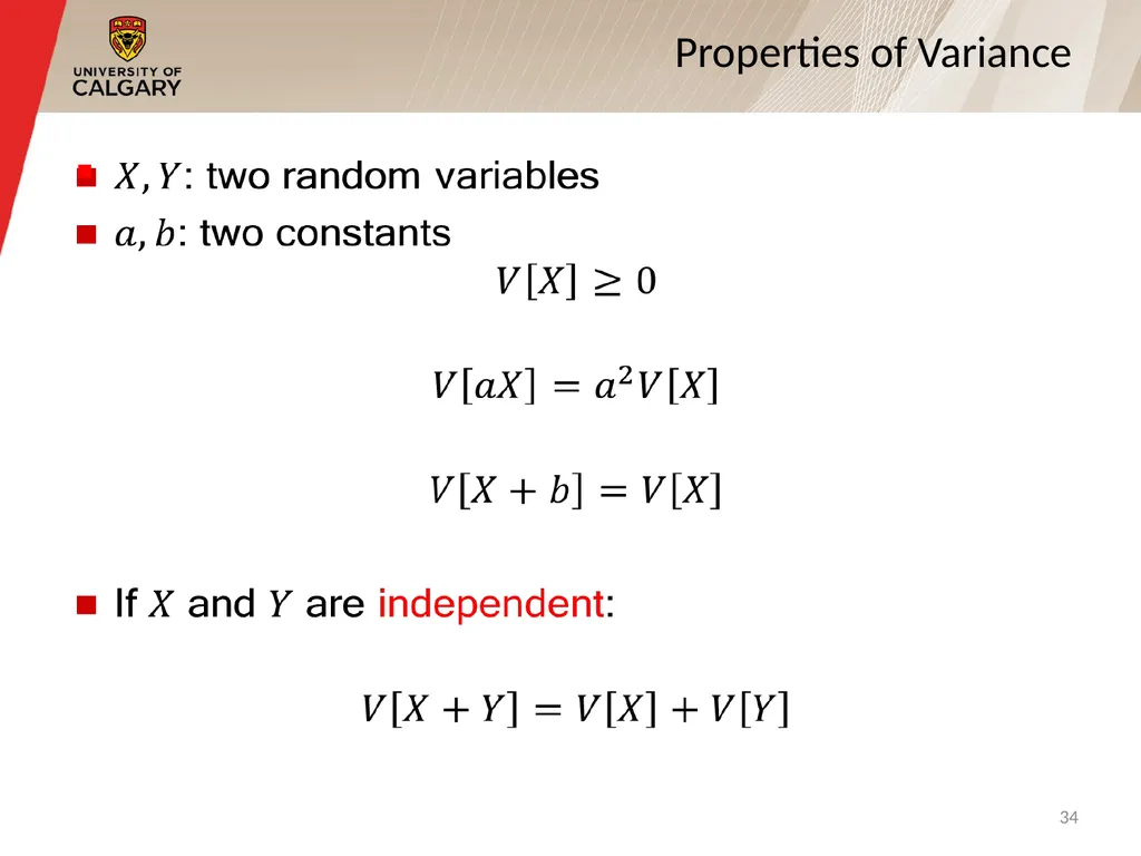
slide34. Properties of Variance 34<br>
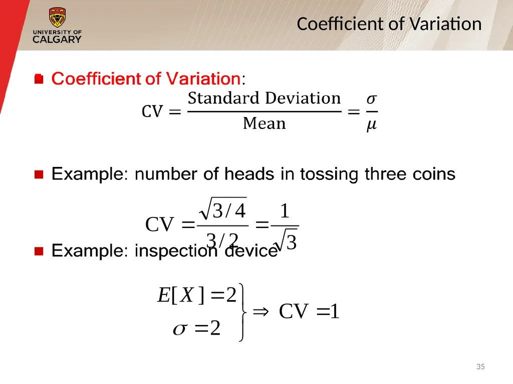
slide35. Coefficient of Variation 35<br>
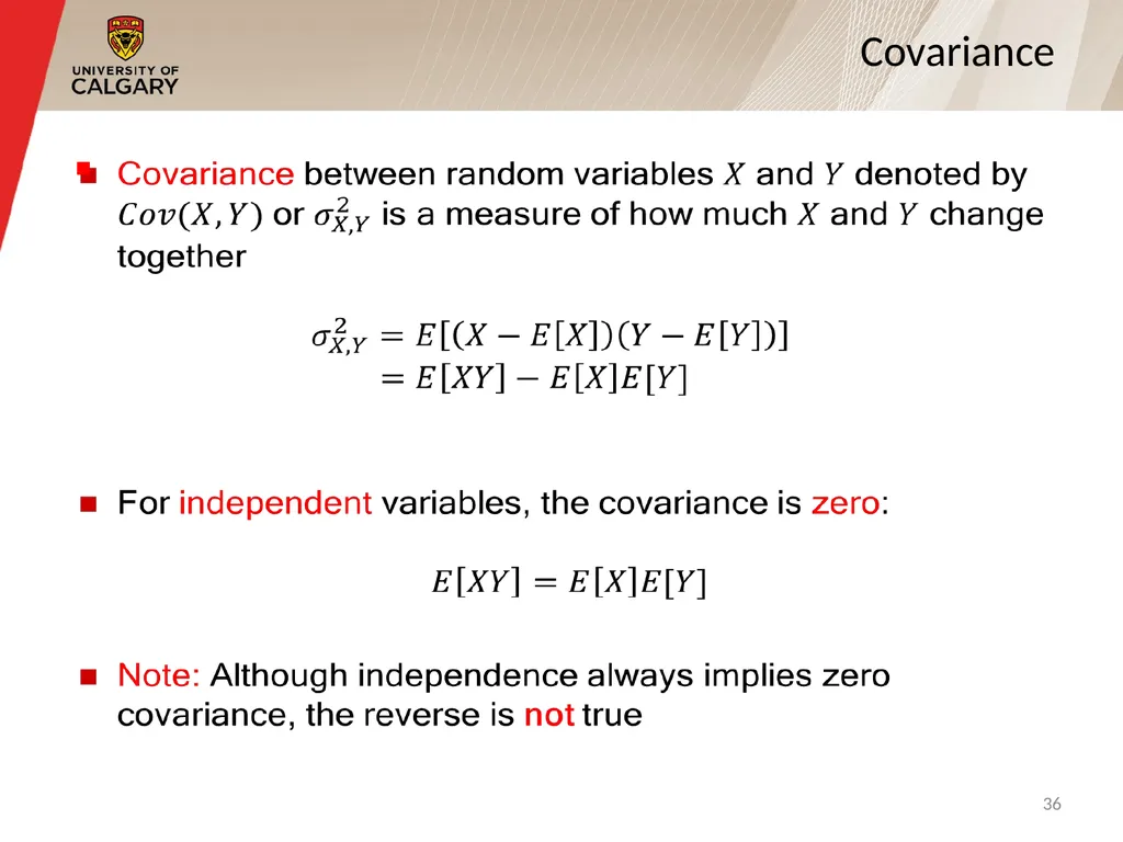
slide36. Covariance 36<br>
slide37. Covariance 37<br>
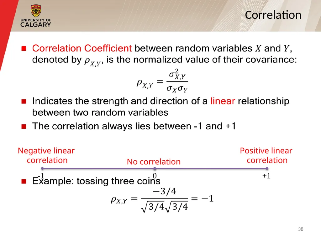
slide38. Correlation 38<br>
slide39. Probability and random variables
Random experiment and random variable
Probability mass/density functions
Expectation, variance, covariance, correlation
Probability distributions
Discrete probability distributions
Continuous probability distributions
Empirical probability distribution Outline 39<br>
slide40. Probability and random variables
Random experiment and random variable
Probability mass/density functions
Expectation, variance, covariance, correlation
Probability distributions
Discrete probability distributions
Continuous probability distributions
Empirical probability distribution Outline 40<br>
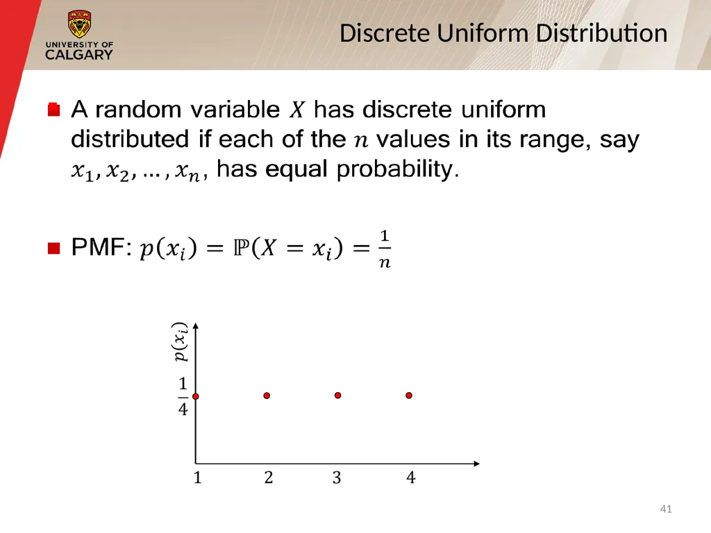
slide41. Discrete Uniform Distribution 41<br>
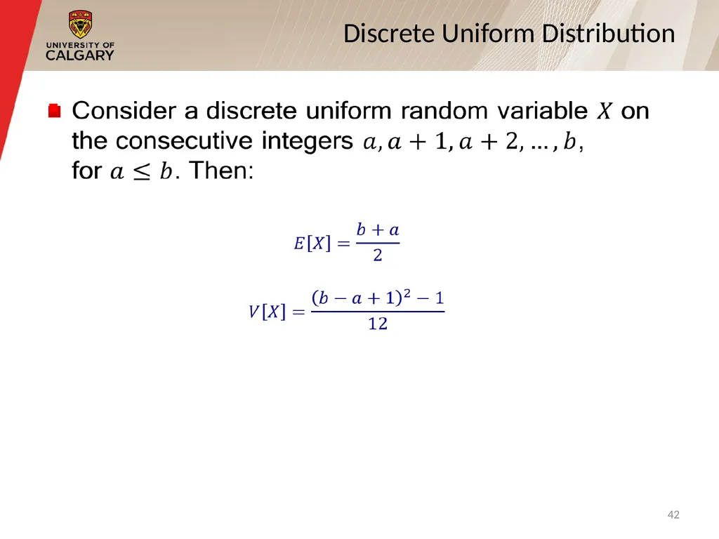
slide42. Discrete Uniform Distribution 42<br>
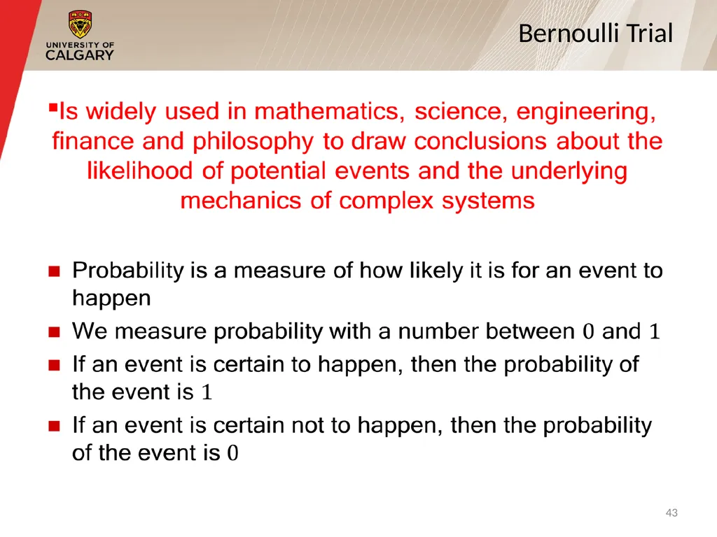
slide43. Bernoulli Trial 43<br>
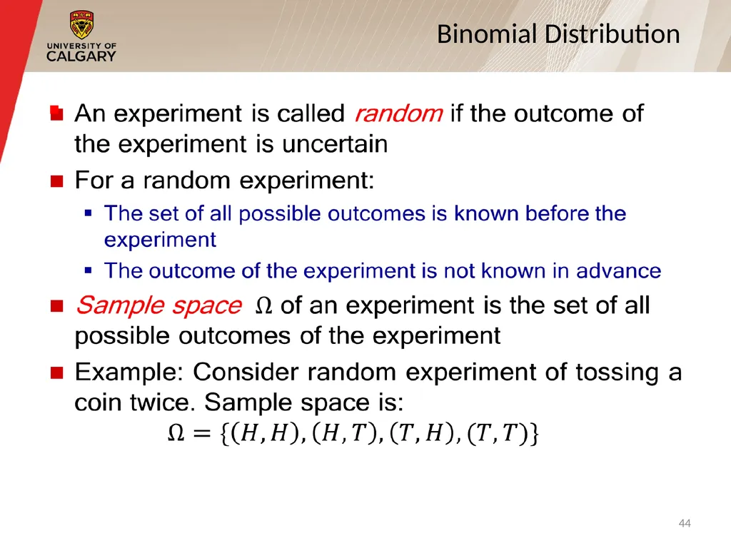
slide44. Binomial Distribution 44<br>
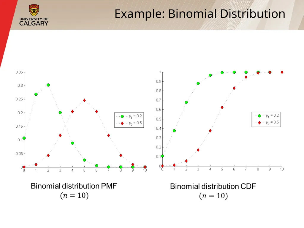
slide45. Example: Binomial Distribution<br>
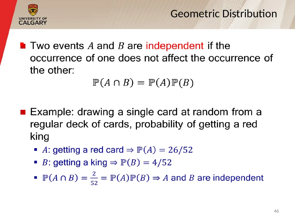
slide46. Geometric Distribution 46<br>
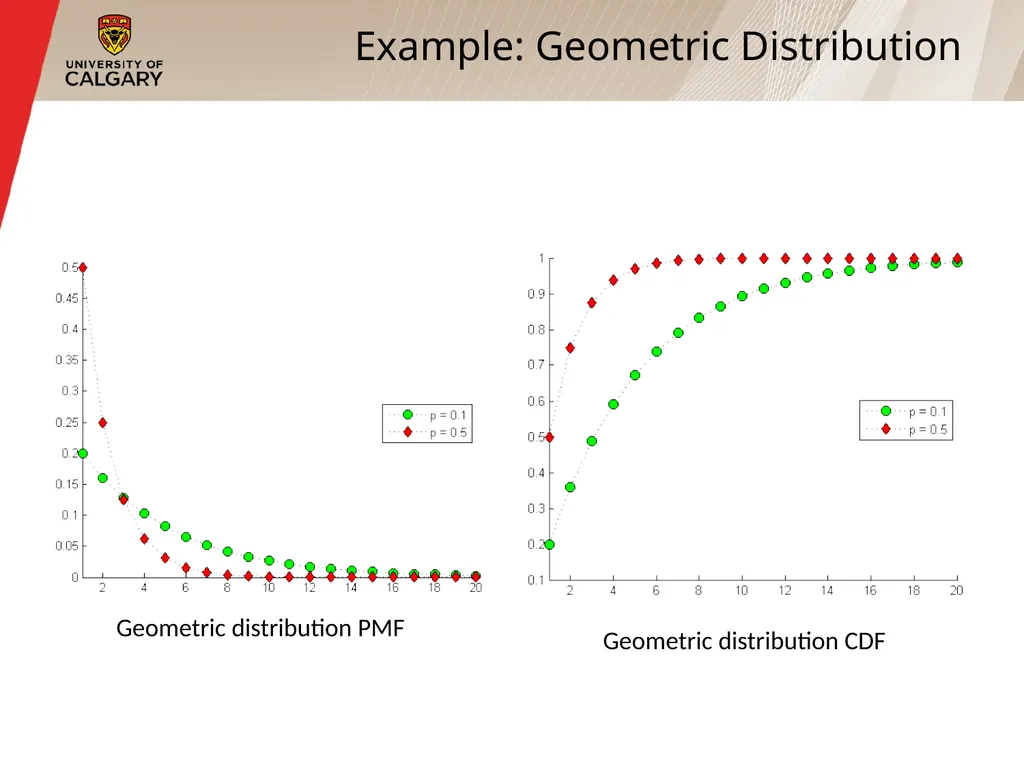
slide47. Example: Geometric Distribution Geometric distribution PMF Geometric distribution CDF<br>
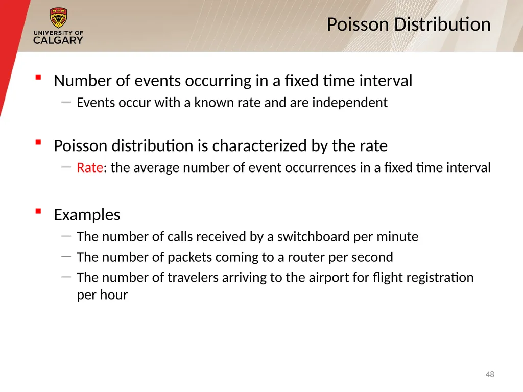
slide48. Number of events occurring in a fixed time interval
Events occur with a known rate and are independent
Poisson distribution is characterized by the rate
Rate: the average number of event occurrences in a fixed time interval
Examples
The number of calls received by a switchboard per minute
The number of packets coming to a router per second
The number of travelers arriving to the airport for flight registration per hour Poisson Distribution 48<br>
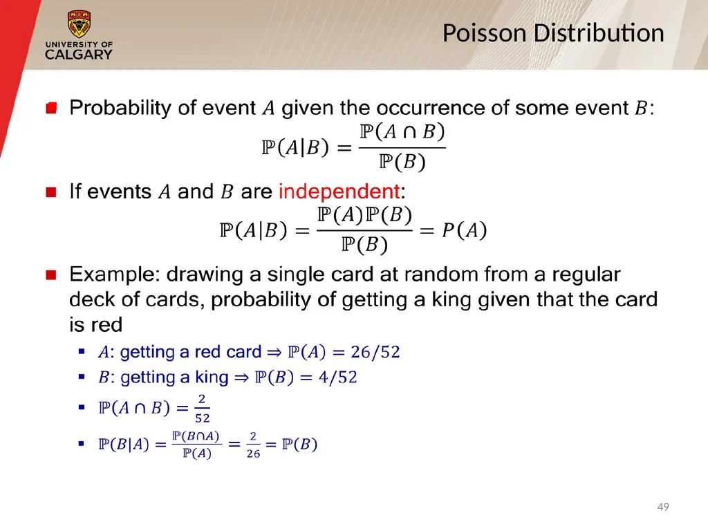
slide49. Poisson Distribution 49<br>
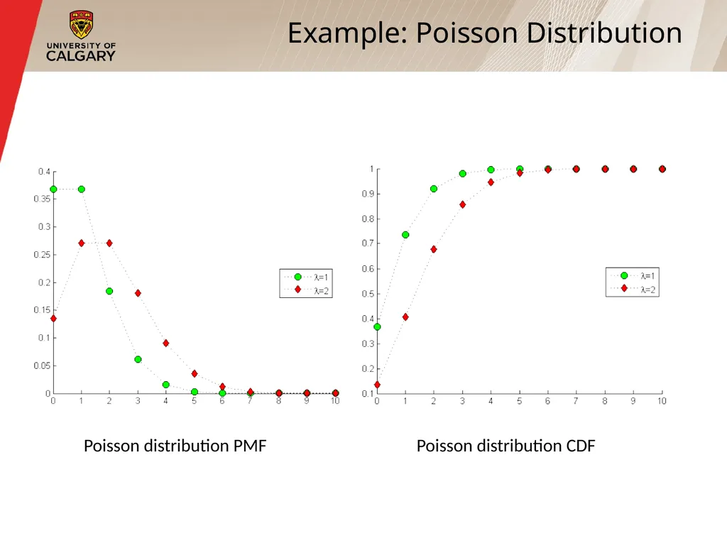
slide50. Example: Poisson Distribution Poisson distribution PMF Poisson distribution CDF<br>
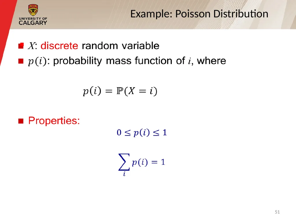
slide51. Example: Poisson Distribution 51<br>
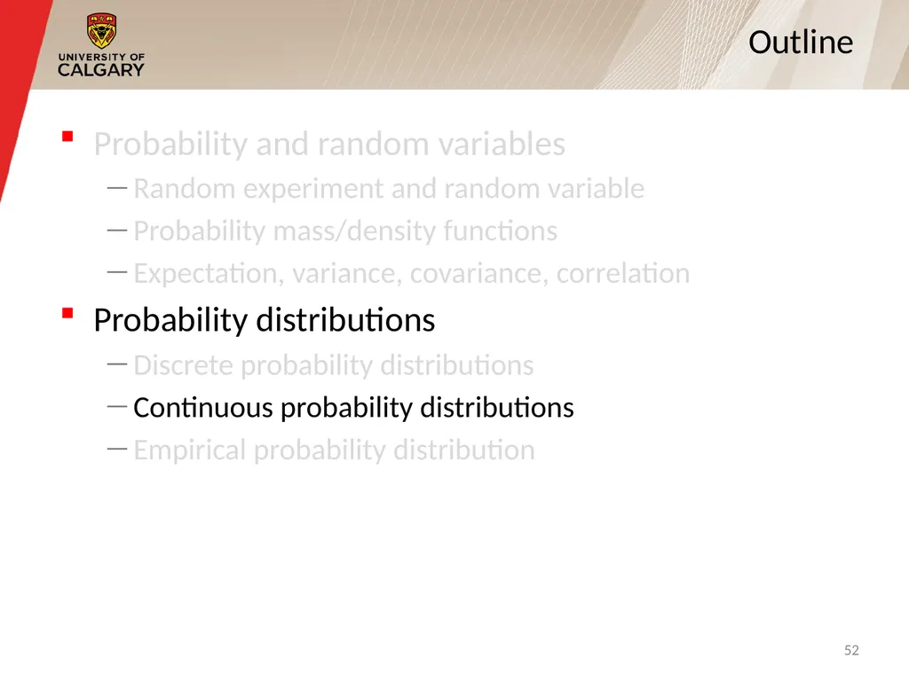
slide52. Probability and random variables
Random experiment and random variable
Probability mass/density functions
Expectation, variance, covariance, correlation
Probability distributions
Discrete probability distributions
Continuous probability distributions
Empirical probability distribution Outline 52<br>
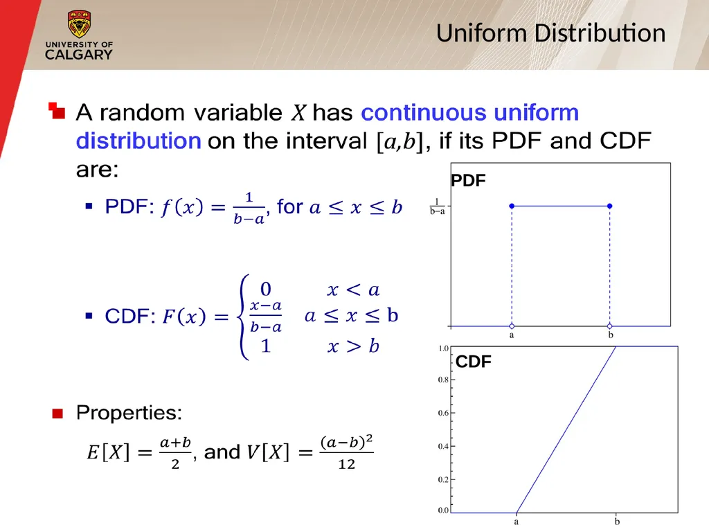
slide53. Uniform Distribution CDF PDF 53<br>
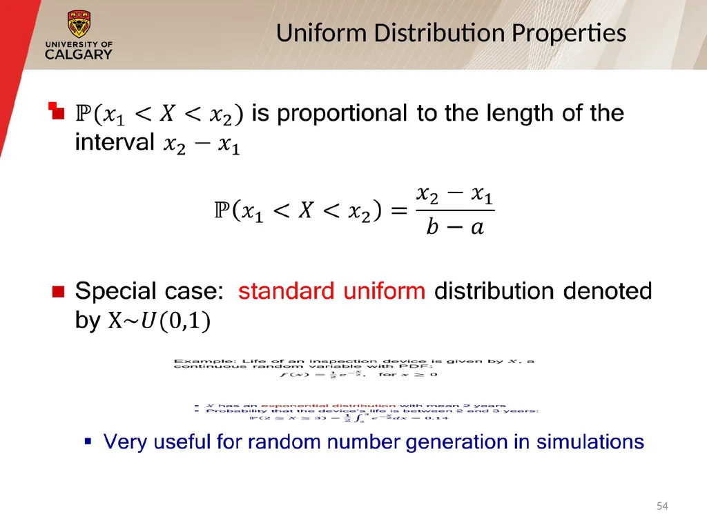
slide54. Uniform Distribution Properties 54<br>
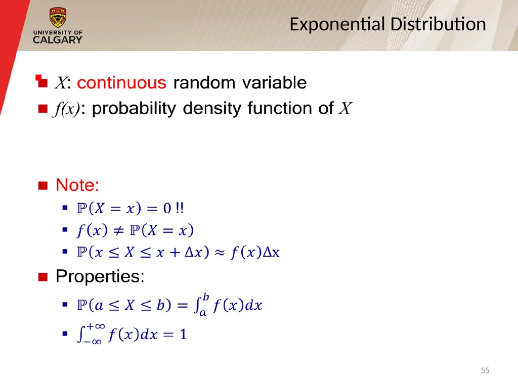
slide55. Exponential Distribution 55<br>
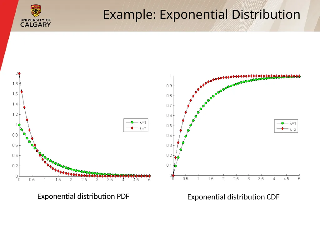
slide56. Example: Exponential Distribution Exponential distribution PDF Exponential distribution CDF<br>
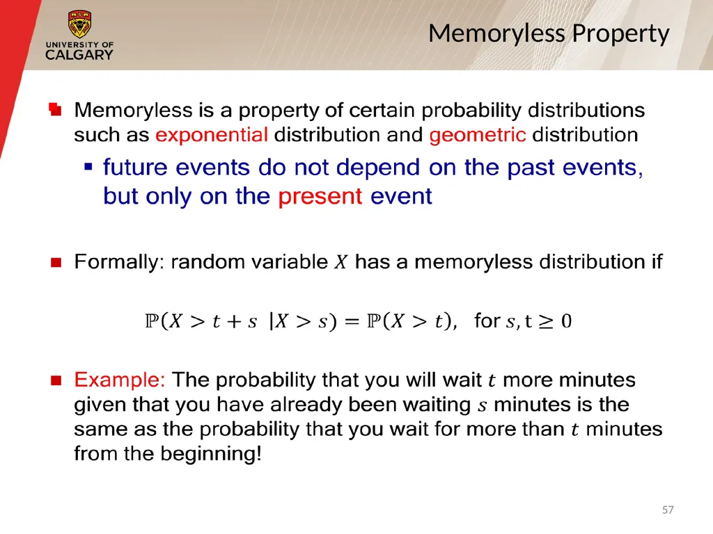
slide57. Memoryless Property 57<br>
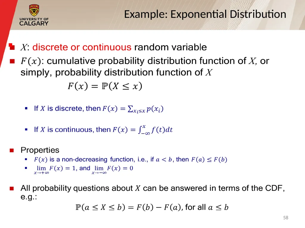
slide58. Example: Exponential Distribution 58<br>
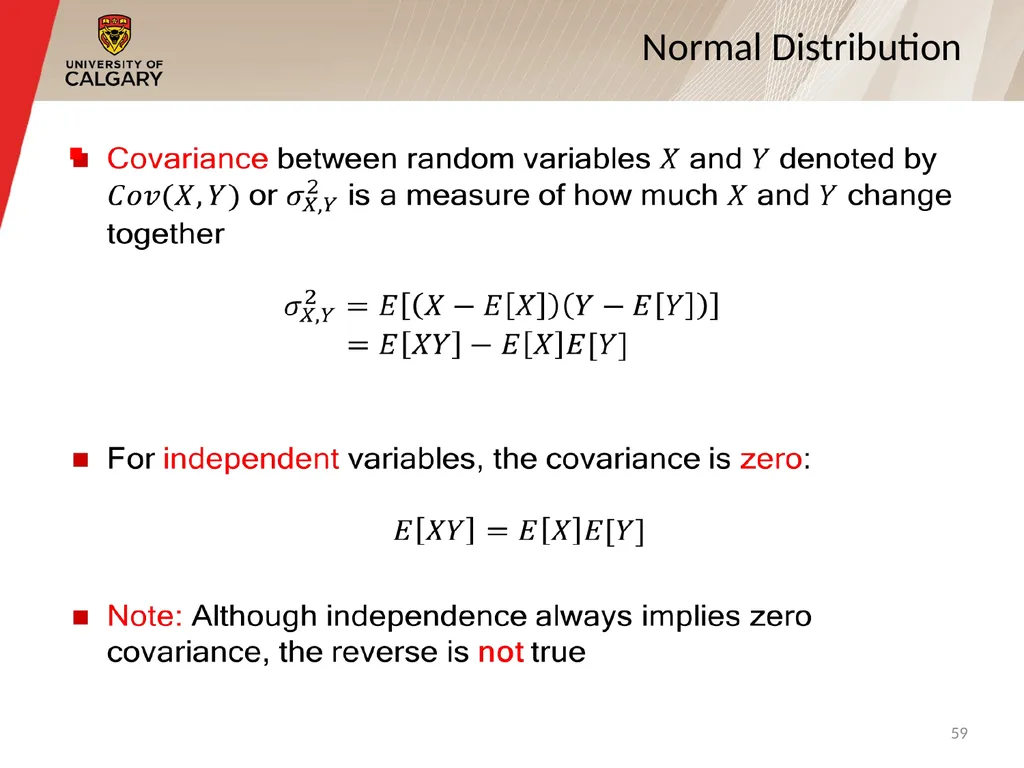
slide59. Normal Distribution 59<br>
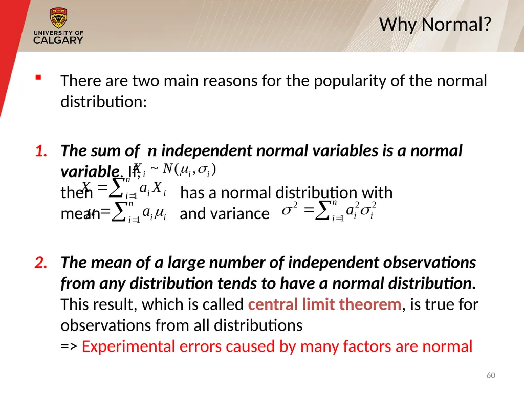
slide60. There are two main reasons for the popularity of the normal distribution:
The sum of n independent normal variables is a normal variable. If, then has a normal distribution with mean and variance
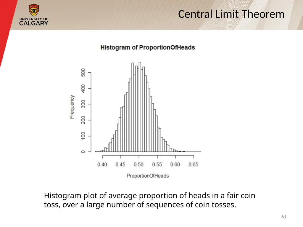
The mean of a large number of independent observations from any distribution tends to have a normal distribution. This result, which is called central limit theorem, is true for observations from all distributions => Experimental errors caused by many factors are normal Why Normal? 60<br>
slide61. Central Limit Theorem Histogram plot of average proportion of heads in a fair coin
toss, over a large number of sequences of coin tosses. 61<br>
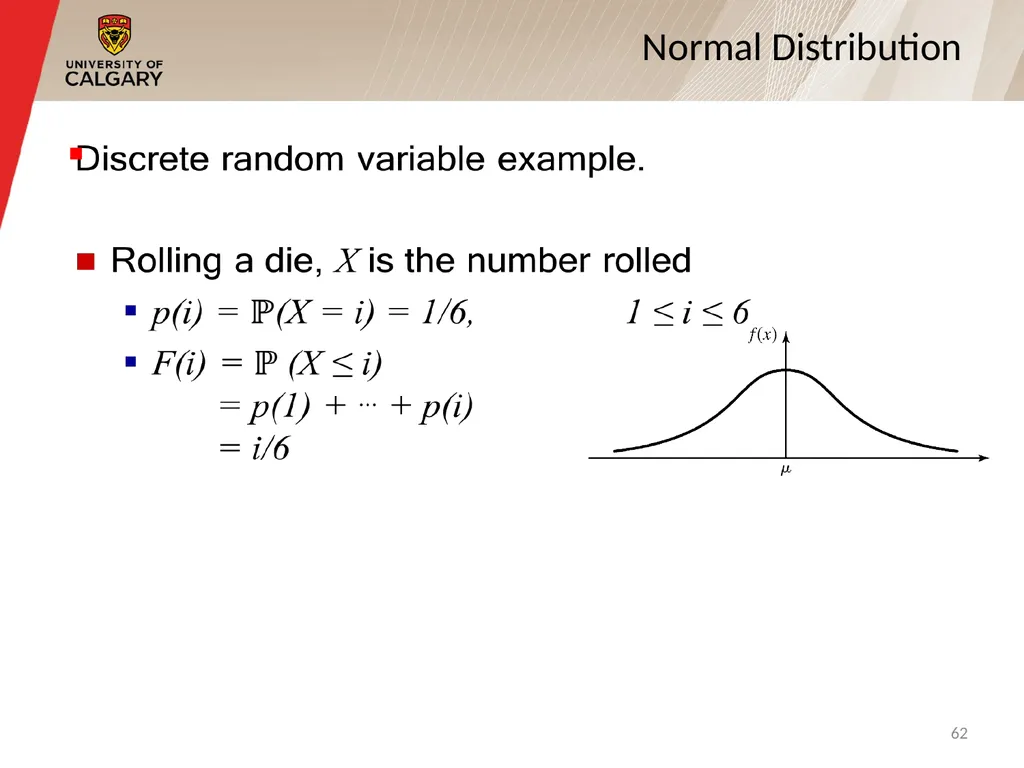
slide62. Normal Distribution 62<br>
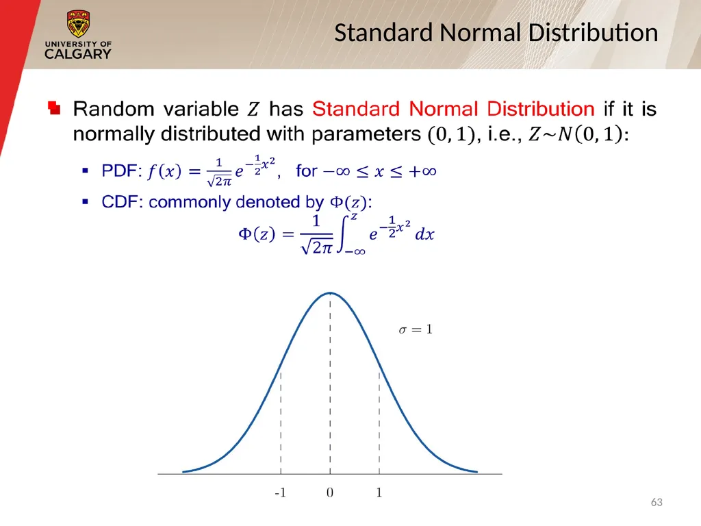
slide63. Standard Normal Distribution 63<br>
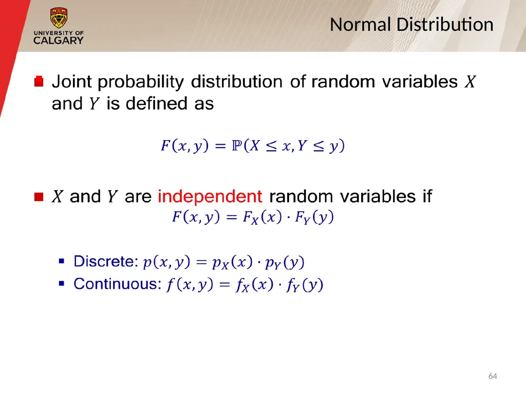
slide64. Normal Distribution 64<br>
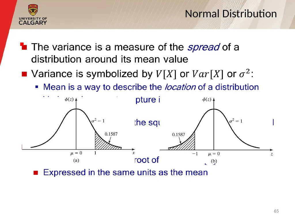
slide65. Normal Distribution 65<br>
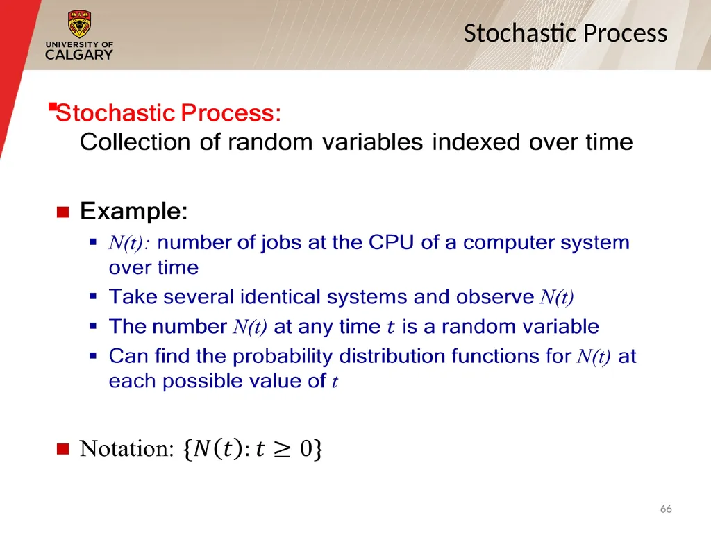
slide66. Stochastic Process 66<br>
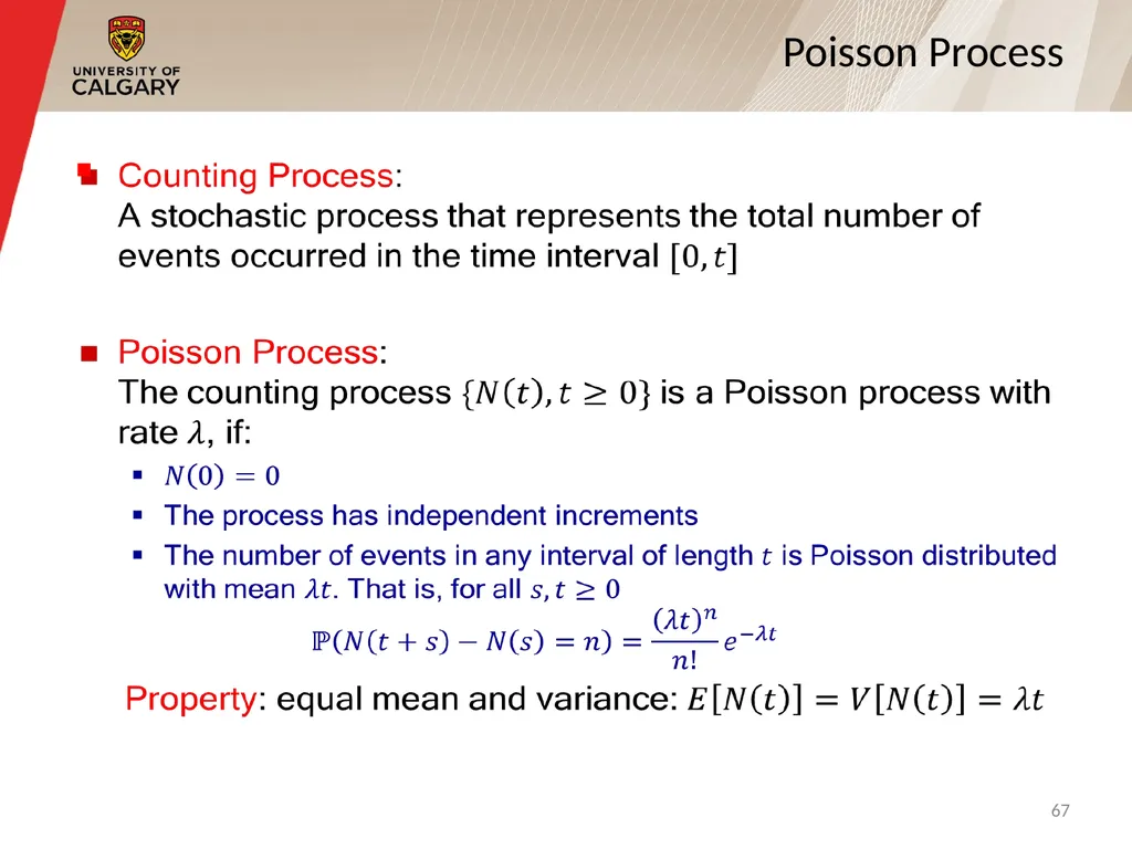
slide67. Poisson Process 67<br>
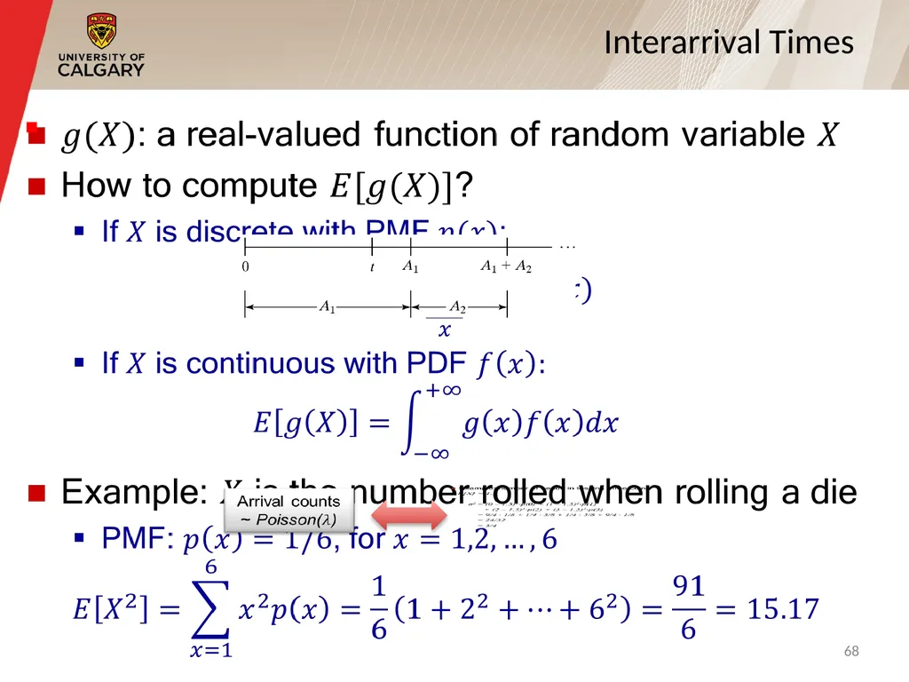
slide68. Interarrival Times 68<br>
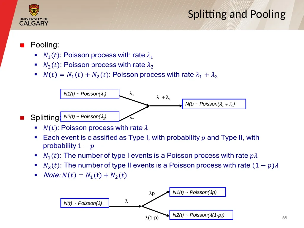
slide69. Splitting and Pooling 69<br>
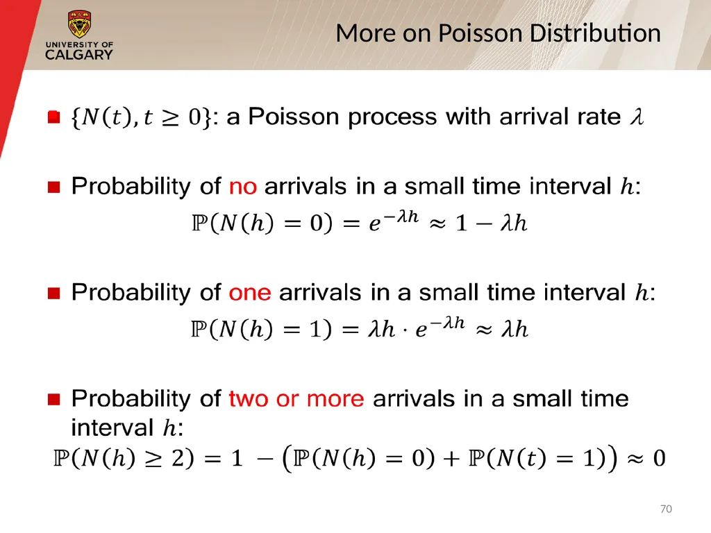
slide70. More on Poisson Distribution 70<br>
slide71. Probability and random variables
Random experiment and random variable
Probability mass/density functions
Expectation, variance, covariance, correlation
Probability distributions
Discrete probability distributions
Continuous probability distributions
Empirical probability distribution Outline 71<br>
slide72. A distribution whose parameters are the observed values in a sample of data:
Could be used if no theoretical distributions fit the data adequately
Advantage: no assumption beyond the observed values in the sample
Disadvantage: sample might not cover the entire range of possible values Empirical Distribution 72<br>
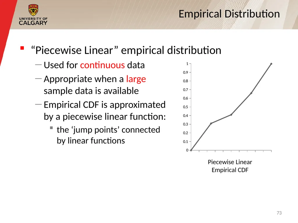
slide73. “Piecewise Linear” empirical distribution
Used for continuous data
Appropriate when a large sample data is available
Empirical CDF is approximated by a piecewise linear function:
the ‘jump points’ connected by linear functions Empirical Distribution Piecewise Linear Empirical CDF 73<br>
slide74. Empirical Distribution 74<br>
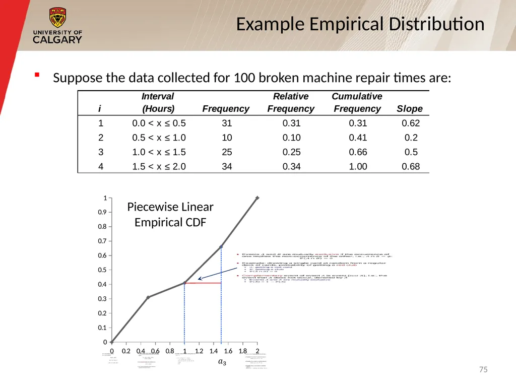
slide75. Suppose the data collected for 100 broken machine repair times are: Example Empirical Distribution Piecewise Linear Empirical CDF 75<br>
Department of Computer Science
University of Calgary
Fall 2017<br>
slide2. The world a model-builder sees is probabilistic rather than deterministic:
Some probability model might well describe the variations
Goals:
Review the fundamental concepts of probability
Understand the difference between discrete and continuous random variable
Review the most common probability models Overview 2<br>
slide3. Probability and random variables
Random experiment and random variable
Probability mass/density functions
Expectation, variance, covariance, correlation
Probability distributions
Discrete probability distributions
Continuous probability distributions
Empirical probability distributions Outline 3<br>
slide4. Probability and random variables
Random experiment and random variable
Probability mass/density functions
Expectation, variance, covariance, correlation
Probability distributions
Discrete probability distributions
Continuous probability distributions
Empirical probability distribution Outline 4<br>
slide5. Probability 5<br>
slide6. Random Experiment 6<br>
slide7. Probability of Events 7<br>
slide8. Joint Probability 8<br>
slide9. Independent Events 9<br>
slide10. Mutually Exclusive Events 10<br>
slide11. Union Probability 11<br>
slide12. Conditional Probability 12<br>
slide13. A numerical value can be associated with each outcome of an experiment
A random variable X is a function from the sample space to the real line that assigns a real number X(s) to each element s of
X: → R
Random variable takes on its values with some probability Random Variable 13<br>
slide14. Example: Consider random experiment of tossing a coin twice. Sample space is:
= {(H,H), (H,T), (T,H), (T,T)}
Define random variable X as the number of heads in the experiment:
X((T,T)) = 0, X((H,T))=1,
X((T,H)) = 1, X((H,H))=2
Example: Rolling a die. Sample space = {1,2,3,4,5,6).
Define random variable X as the number rolled:
X(j) = j, 1 ≤ j ≤ 6 Random Variable 14<br>
slide15. Example: roll two fair dice and observe the outcome
Sample space = {(i,j) | 1 ≤ i ≤ 6, 1 ≤ j ≤ 6}
i: integer from the first die
j: integer from the second die Random Variable Possible outcomes 15<br>
slide16. Random Variable 16<br>
slide17. Discrete
Random variables whose set of possible values can be written as a finite or infinite sequence
Example: number of requests sent to a web server
Continuous
Random variables that take a continuum of possible values
Example: time between requests sent to a web server Types of Random Variables 17<br>
slide18. Probability Mass Function (PMF) 18<br>
slide19. PMF Examples 19<br>
slide20. Probability Density Function (PDF) 20<br>
slide21. Probability Density Function 21<br>
slide22. Cumulative Distribution Function (CDF) 22<br>
slide23. Cumulative Distribution Function 23<br>
slide24. Cumulative Distribution Function 24<br>
slide25. Joint Probability Distribution 25<br>
slide26. Expectation of a Random Variable 26<br>
slide27. Expectation of a Function 27<br>
slide28. Properties of Expectation 28<br>
slide29. Multiplying means to get the mean of a product
Example: tossing three coins
X: number of heads
Y: number of tails
E[X] = E[Y] = 3/2 E[X]E[Y] = 9/4
E[XY] = 3/2
E[XY] ≠ E[X]E[Y]
Dividing means to get the mean of a ratio Misuses of Expectations 29<br>
slide30. Variance of a Random Variable 30<br>
slide31. Variance: The expected value of the square of distance between a random variable and its mean
where, μ= E[X]
Equivalently:
σ2 = E[X2] – (E[X])2 Variance of a Random Variable 31<br>
slide32. Variance of a Random Variable 32<br>
slide33. Variance of a Random Variable 33<br>
slide34. Properties of Variance 34<br>
slide35. Coefficient of Variation 35<br>
slide36. Covariance 36<br>
slide37. Covariance 37<br>
slide38. Correlation 38<br>
slide39. Probability and random variables
Random experiment and random variable
Probability mass/density functions
Expectation, variance, covariance, correlation
Probability distributions
Discrete probability distributions
Continuous probability distributions
Empirical probability distribution Outline 39<br>
slide40. Probability and random variables
Random experiment and random variable
Probability mass/density functions
Expectation, variance, covariance, correlation
Probability distributions
Discrete probability distributions
Continuous probability distributions
Empirical probability distribution Outline 40<br>
slide41. Discrete Uniform Distribution 41<br>
slide42. Discrete Uniform Distribution 42<br>
slide43. Bernoulli Trial 43<br>
slide44. Binomial Distribution 44<br>
slide45. Example: Binomial Distribution<br>
slide46. Geometric Distribution 46<br>
slide47. Example: Geometric Distribution Geometric distribution PMF Geometric distribution CDF<br>
slide48. Number of events occurring in a fixed time interval
Events occur with a known rate and are independent
Poisson distribution is characterized by the rate
Rate: the average number of event occurrences in a fixed time interval
Examples
The number of calls received by a switchboard per minute
The number of packets coming to a router per second
The number of travelers arriving to the airport for flight registration per hour Poisson Distribution 48<br>
slide49. Poisson Distribution 49<br>
slide50. Example: Poisson Distribution Poisson distribution PMF Poisson distribution CDF<br>
slide51. Example: Poisson Distribution 51<br>
slide52. Probability and random variables
Random experiment and random variable
Probability mass/density functions
Expectation, variance, covariance, correlation
Probability distributions
Discrete probability distributions
Continuous probability distributions
Empirical probability distribution Outline 52<br>
slide53. Uniform Distribution CDF PDF 53<br>
slide54. Uniform Distribution Properties 54<br>
slide55. Exponential Distribution 55<br>
slide56. Example: Exponential Distribution Exponential distribution PDF Exponential distribution CDF<br>
slide57. Memoryless Property 57<br>
slide58. Example: Exponential Distribution 58<br>
slide59. Normal Distribution 59<br>
slide60. There are two main reasons for the popularity of the normal distribution:
The sum of n independent normal variables is a normal variable. If, then has a normal distribution with mean and variance
The mean of a large number of independent observations from any distribution tends to have a normal distribution. This result, which is called central limit theorem, is true for observations from all distributions => Experimental errors caused by many factors are normal Why Normal? 60<br>
slide61. Central Limit Theorem Histogram plot of average proportion of heads in a fair coin
toss, over a large number of sequences of coin tosses. 61<br>
slide62. Normal Distribution 62<br>
slide63. Standard Normal Distribution 63<br>
slide64. Normal Distribution 64<br>
slide65. Normal Distribution 65<br>
slide66. Stochastic Process 66<br>
slide67. Poisson Process 67<br>
slide68. Interarrival Times 68<br>
slide69. Splitting and Pooling 69<br>
slide70. More on Poisson Distribution 70<br>
slide71. Probability and random variables
Random experiment and random variable
Probability mass/density functions
Expectation, variance, covariance, correlation
Probability distributions
Discrete probability distributions
Continuous probability distributions
Empirical probability distribution Outline 71<br>
slide72. A distribution whose parameters are the observed values in a sample of data:
Could be used if no theoretical distributions fit the data adequately
Advantage: no assumption beyond the observed values in the sample
Disadvantage: sample might not cover the entire range of possible values Empirical Distribution 72<br>
slide73. “Piecewise Linear” empirical distribution
Used for continuous data
Appropriate when a large sample data is available
Empirical CDF is approximated by a piecewise linear function:
the ‘jump points’ connected by linear functions Empirical Distribution Piecewise Linear Empirical CDF 73<br>
slide74. Empirical Distribution 74<br>
slide75. Suppose the data collected for 100 broken machine repair times are: Example Empirical Distribution Piecewise Linear Empirical CDF 75<br>