
Discrete Choice Modeling William Greene Stern
T
Published · 79 slides · 0 views

1 / 1









Description
Discrete Choice Modeling William Greene Stern School of Business New York University 0 Introduction 1 Summary 2 Binary Choice 3 Panel Data 4 Bivariate Probit 5 Ordered Choice 6 Count Data 7 Multinomial Choice 8 Nested Logit 9 Heterogeneity
Related Topics
Share
Embed code
Download this presentation From Below
"Discrete Choice Modeling William Greene Stern" is the property of its rightful owner. Permission is granted to download and print the materials on this website for personal, non-commercial use only, and to display it on your personal computer provided you do not modify the materials and that you retain all copyright notices contained in the materials. By downloading content from our website, you accept the terms of this agreement.
Presentation Transcript
01
Discrete Choice Modeling William Greene
Stern School of Business
New York University 0 Introduction
1 Summary
2 Binary Choice
3 Panel Data
4 Bivariate Probit
5 Ordered Choice
6 Count Data
7 Multinomial Choice
8 Nested Logit
9 Heterogeneity
10 Latent Class
11 Mixed Logit
12 Stated Preference
13 Hybrid Choice<br>
Stern School of Business
New York University 0 Introduction
1 Summary
2 Binary Choice
3 Panel Data
4 Bivariate Probit
5 Ordered Choice
6 Count Data
7 Multinomial Choice
8 Nested Logit
9 Heterogeneity
10 Latent Class
11 Mixed Logit
12 Stated Preference
13 Hybrid Choice<br>
02
What’s Wrong with the MNL Model? Insufficiently heterogeneous:
“… economists are often more interested in aggregate effects and regard heterogeneity as a statistical nuisance parameter problem which must be addressed but not emphasized. Econometricians frequently employ methods which do not allow for the estimation of individual level parameters.” (Allenby and Rossi, Journal of Econometrics, 1999)<br>
“… economists are often more interested in aggregate effects and regard heterogeneity as a statistical nuisance parameter problem which must be addressed but not emphasized. Econometricians frequently employ methods which do not allow for the estimation of individual level parameters.” (Allenby and Rossi, Journal of Econometrics, 1999)<br>
03
Several Types of Heterogeneity Differences across choice makers
Observable: Usually demographics such as age, sex
Unobservable: Usually modeled as ‘random effects’
Choice strategy: How consumers make decisions. (E.g., omitted attributes)
Preference Structure: Model frameworks such as latent class structures
Preferences: Model ‘parameters’
Discrete variation – latent class
Continuous variation – mixed models
Discrete-Continuous variation<br>
Observable: Usually demographics such as age, sex
Unobservable: Usually modeled as ‘random effects’
Choice strategy: How consumers make decisions. (E.g., omitted attributes)
Preference Structure: Model frameworks such as latent class structures
Preferences: Model ‘parameters’
Discrete variation – latent class
Continuous variation – mixed models
Discrete-Continuous variation<br>
04
Heterogeneity in Choice Strategy Consumers avoid ‘complexity’
Lexicographic preferences eliminate certain choices choice set may be endogenously determined
Simplification strategies may eliminate certain attributes
Information processing strategy is a source of heterogeneity in the model.<br>
Lexicographic preferences eliminate certain choices choice set may be endogenously determined
Simplification strategies may eliminate certain attributes
Information processing strategy is a source of heterogeneity in the model.<br>
05
Accommodating Heterogeneity Observed? Enter in the model in
familiar (and unfamiliar) ways.
Unobserved? Takes the form of randomness in the model.<br>
Unobserved? Takes the form of randomness in the model.<br>
06
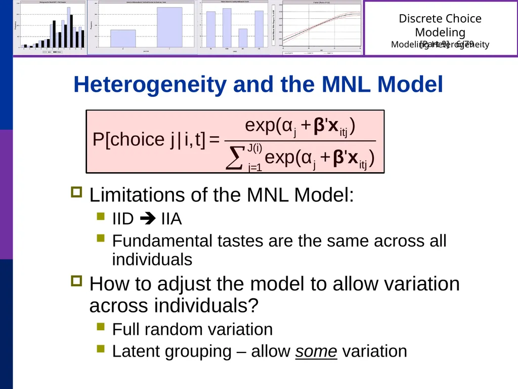
Heterogeneity and the MNL Model Limitations of the MNL Model:
IID IIA
Fundamental tastes are the same across all individuals
How to adjust the model to allow variation across individuals?
Full random variation
Latent grouping – allow some variation<br>
IID IIA
Fundamental tastes are the same across all individuals
How to adjust the model to allow variation across individuals?
Full random variation
Latent grouping – allow some variation<br>
07
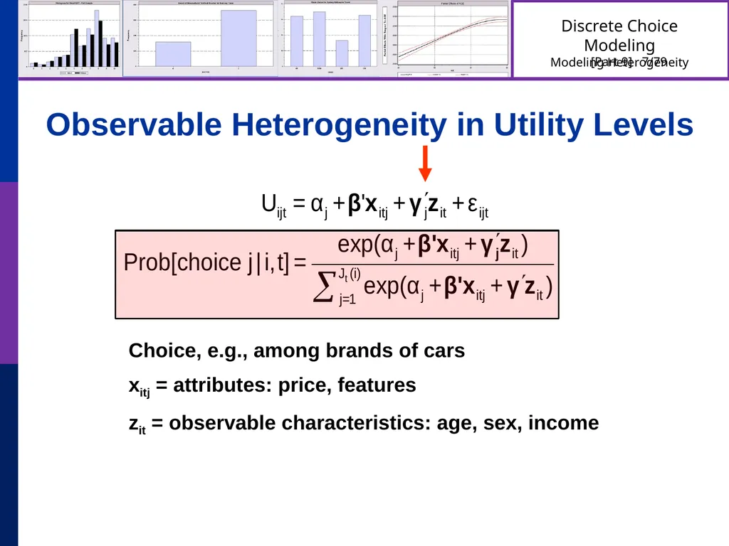
Observable Heterogeneity in Utility Levels Choice, e.g., among brands of cars
xitj = attributes: price, features
zit = observable characteristics: age, sex, income<br>
xitj = attributes: price, features
zit = observable characteristics: age, sex, income<br>
08
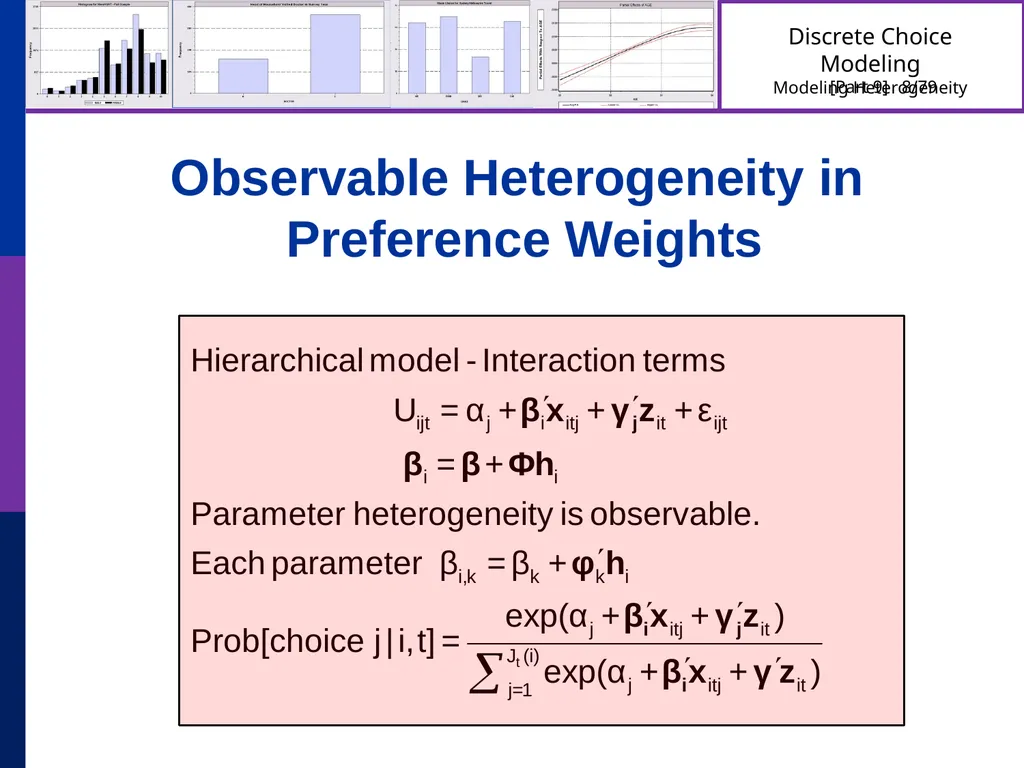
Observable Heterogeneity in
Preference Weights<br>
09
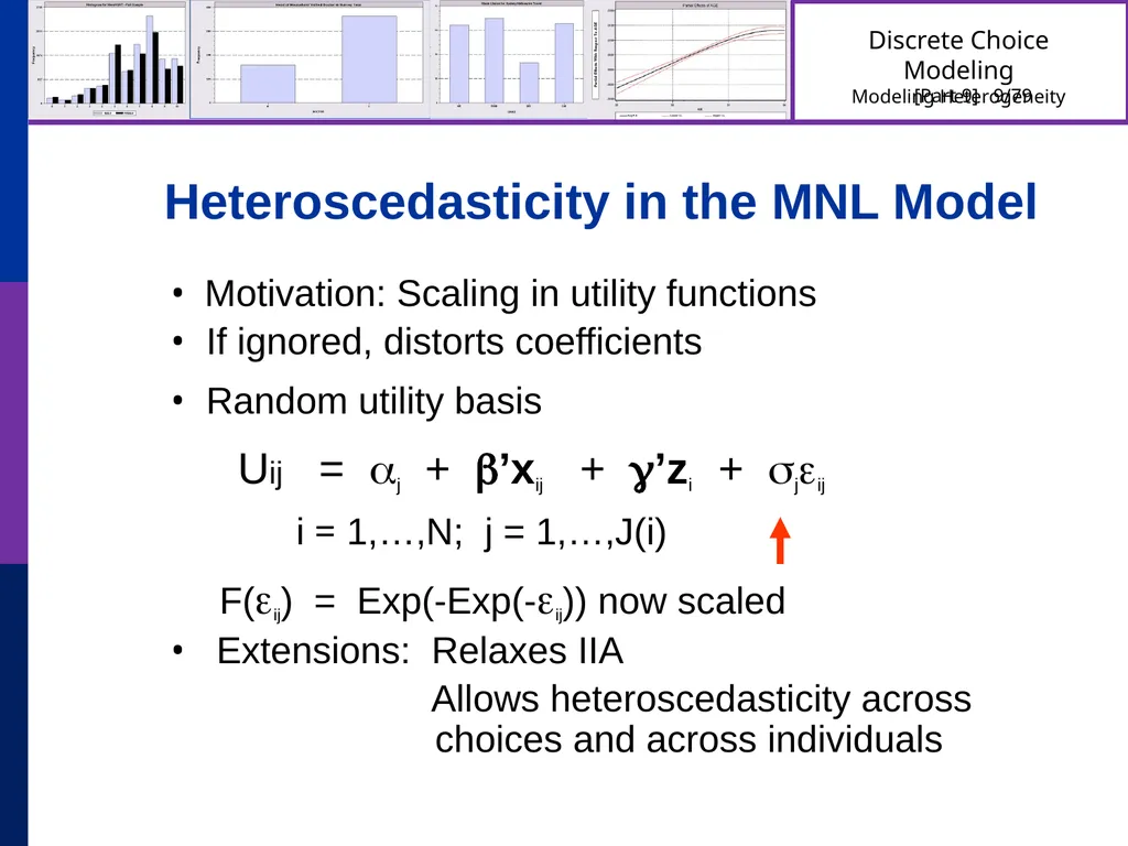
Heteroscedasticity in the MNL Model • Motivation: Scaling in utility functions
• If ignored, distorts coefficients
• Random utility basis
Uij = j + ’xij + ’zi + jij
i = 1,…,N; j = 1,…,J(i)
F(ij) = Exp(-Exp(-ij)) now scaled
• Extensions: Relaxes IIA
Allows heteroscedasticity across choices and across individuals<br>
• If ignored, distorts coefficients
• Random utility basis
Uij = j + ’xij + ’zi + jij
i = 1,…,N; j = 1,…,J(i)
F(ij) = Exp(-Exp(-ij)) now scaled
• Extensions: Relaxes IIA
Allows heteroscedasticity across choices and across individuals<br>
10
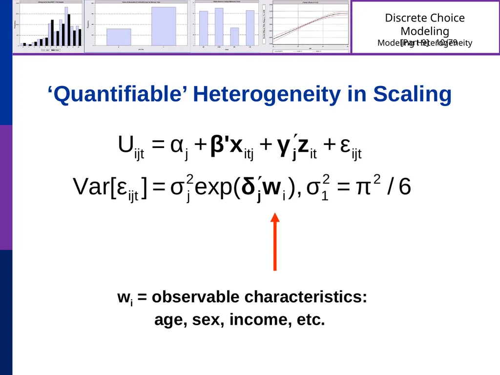
‘Quantifiable’ Heterogeneity in Scaling wi = observable characteristics:
age, sex, income, etc.<br>
11
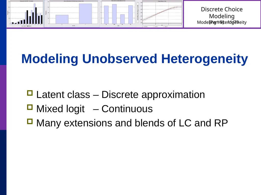
Modeling Unobserved Heterogeneity Latent class – Discrete approximation
Mixed logit – Continuous
Many extensions and blends of LC and RP<br>
Mixed logit – Continuous
Many extensions and blends of LC and RP<br>
12
Latent Class
Models<br>
13
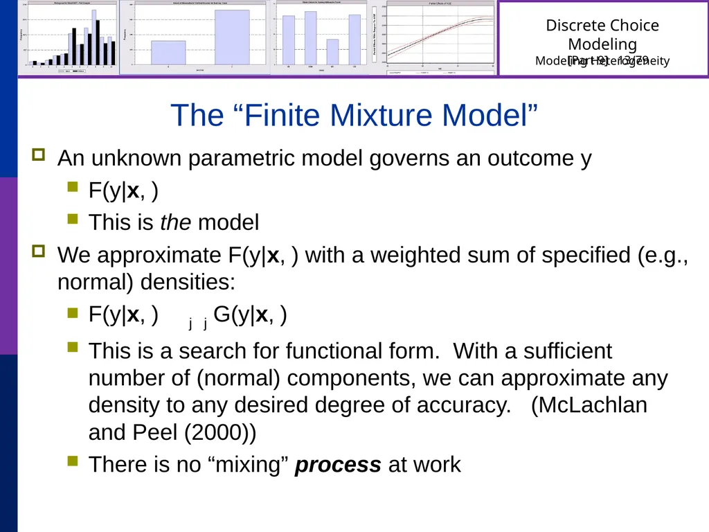
The “Finite Mixture Model” An unknown parametric model governs an outcome y
F(y|x,)
This is the model
We approximate F(y|x,) with a weighted sum of specified (e.g., normal) densities:
F(y|x,) j j G(y|x,)
This is a search for functional form. With a sufficient number of (normal) components, we can approximate any density to any desired degree of accuracy. (McLachlan and Peel (2000))
There is no “mixing” process at work<br>
F(y|x,)
This is the model
We approximate F(y|x,) with a weighted sum of specified (e.g., normal) densities:
F(y|x,) j j G(y|x,)
This is a search for functional form. With a sufficient number of (normal) components, we can approximate any density to any desired degree of accuracy. (McLachlan and Peel (2000))
There is no “mixing” process at work<br>
14
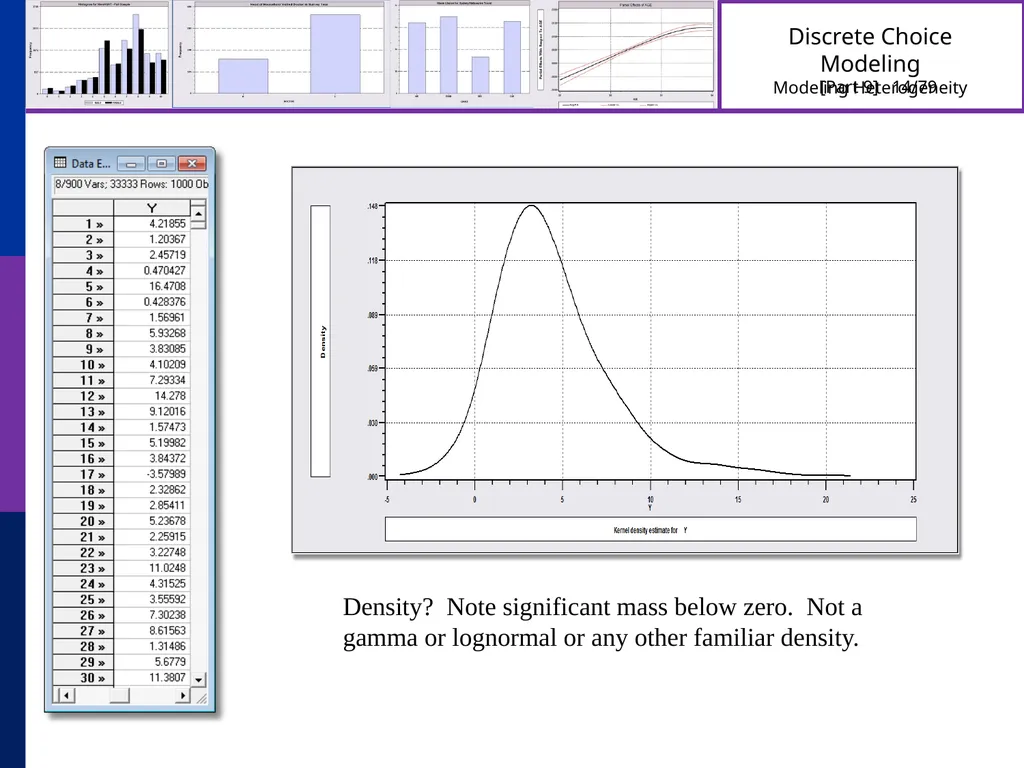
Density? Note significant mass below zero. Not a gamma or lognormal or any other familiar density.<br>
15
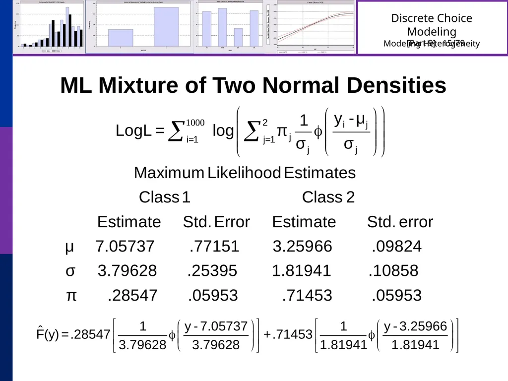
ML Mixture of Two Normal Densities<br>
16
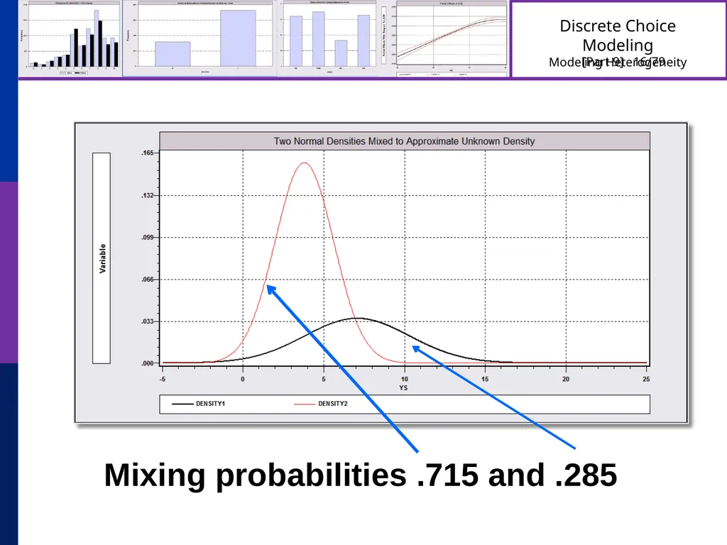
Mixing probabilities .715 and .285<br>
17
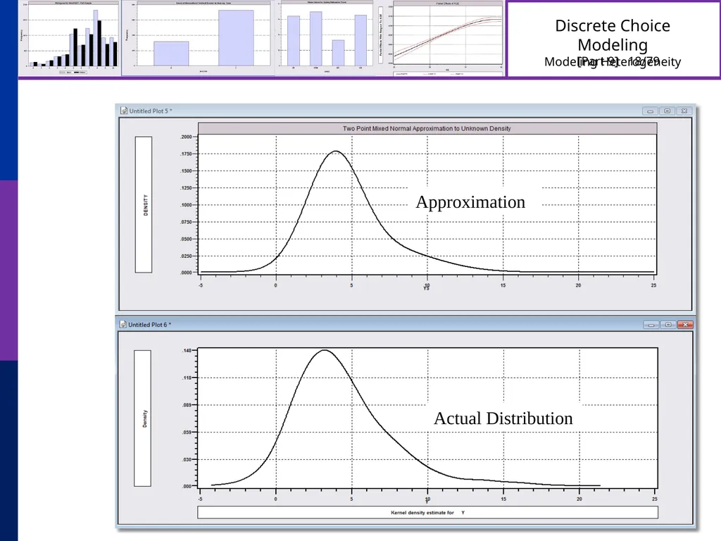
The actual process is a mix of chi squared(5) and normal(3,2) with mixing probabilities .7 and .3.<br>
18
Approximation Actual Distribution<br>
19
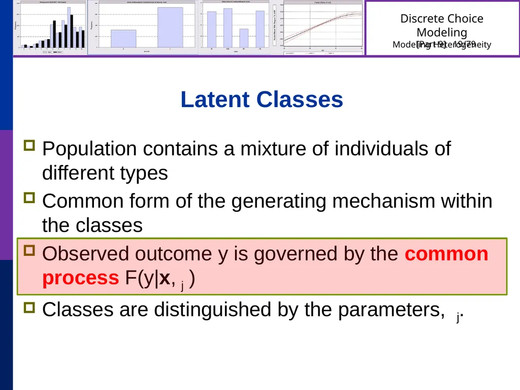
Latent Classes Population contains a mixture of individuals of different types
Common form of the generating mechanism within the classes
Observed outcome y is governed by the common process F(y|x,j )
Classes are distinguished by the parameters, j.<br>
Common form of the generating mechanism within the classes
Observed outcome y is governed by the common process F(y|x,j )
Classes are distinguished by the parameters, j.<br>
20
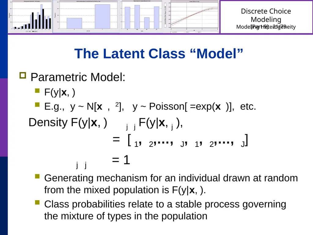
The Latent Class “Model” Parametric Model:
F(y|x,)
E.g., y ~ N[x, 2], y ~ Poisson[=exp(x)], etc.
Density F(y|x,) j j F(y|x,j ), = [1, 2,…, J, 1, 2,…, J]
j j = 1
Generating mechanism for an individual drawn at random from the mixed population is F(y|x,).
Class probabilities relate to a stable process governing the mixture of types in the population<br>
F(y|x,)
E.g., y ~ N[x, 2], y ~ Poisson[=exp(x)], etc.
Density F(y|x,) j j F(y|x,j ), = [1, 2,…, J, 1, 2,…, J]
j j = 1
Generating mechanism for an individual drawn at random from the mixed population is F(y|x,).
Class probabilities relate to a stable process governing the mixture of types in the population<br>
21
RANDOM Parameter
Models<br>
22
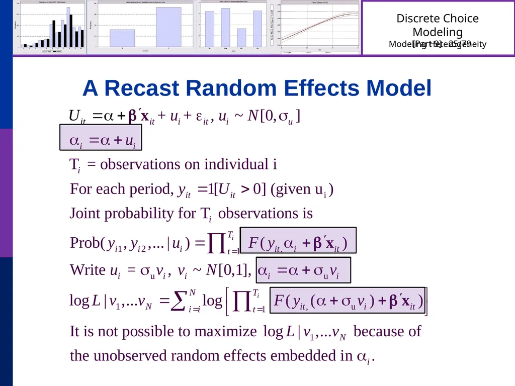
A Recast Random Effects Model<br>
23
A Computable Log Likelihood<br>
24
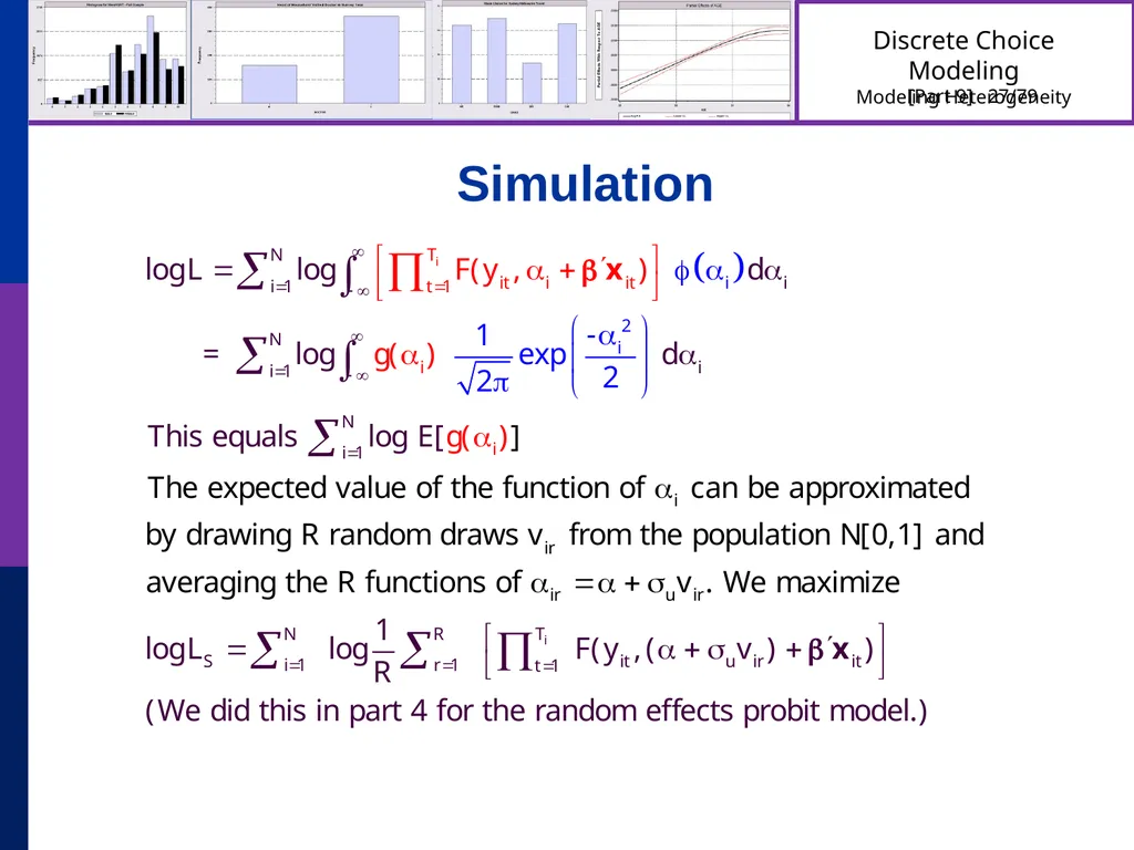
Simulation<br>
25
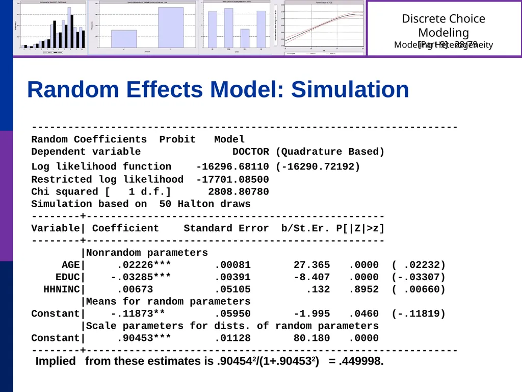
Random Effects Model: Simulation ----------------------------------------------------------------------
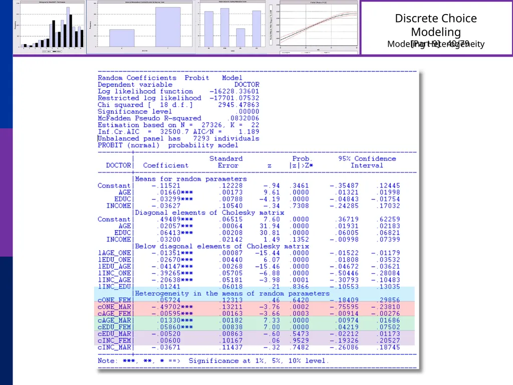
Random Coefficients Probit Model
Dependent variable DOCTOR (Quadrature Based)
Log likelihood function -16296.68110 (-16290.72192)
Restricted log likelihood -17701.08500
Chi squared [ 1 d.f.] 2808.80780
Simulation based on 50 Halton draws
--------+-------------------------------------------------
Variable| Coefficient Standard Error b/St.Er. P[|Z|>z]
--------+-------------------------------------------------
|Nonrandom parameters
AGE| .02226*** .00081 27.365 .0000 ( .02232)
EDUC| -.03285*** .00391 -8.407 .0000 (-.03307)
HHNINC| .00673 .05105 .132 .8952 ( .00660)
|Means for random parameters
Constant| -.11873** .05950 -1.995 .0460 (-.11819)
|Scale parameters for dists. of random parameters
Constant| .90453*** .01128 80.180 .0000
--------+------------------------------------------------------------- Implied from these estimates is .904542/(1+.904532) = .449998.<br>
Random Coefficients Probit Model
Dependent variable DOCTOR (Quadrature Based)
Log likelihood function -16296.68110 (-16290.72192)
Restricted log likelihood -17701.08500
Chi squared [ 1 d.f.] 2808.80780
Simulation based on 50 Halton draws
--------+-------------------------------------------------
Variable| Coefficient Standard Error b/St.Er. P[|Z|>z]
--------+-------------------------------------------------
|Nonrandom parameters
AGE| .02226*** .00081 27.365 .0000 ( .02232)
EDUC| -.03285*** .00391 -8.407 .0000 (-.03307)
HHNINC| .00673 .05105 .132 .8952 ( .00660)
|Means for random parameters
Constant| -.11873** .05950 -1.995 .0460 (-.11819)
|Scale parameters for dists. of random parameters
Constant| .90453*** .01128 80.180 .0000
--------+------------------------------------------------------------- Implied from these estimates is .904542/(1+.904532) = .449998.<br>
26
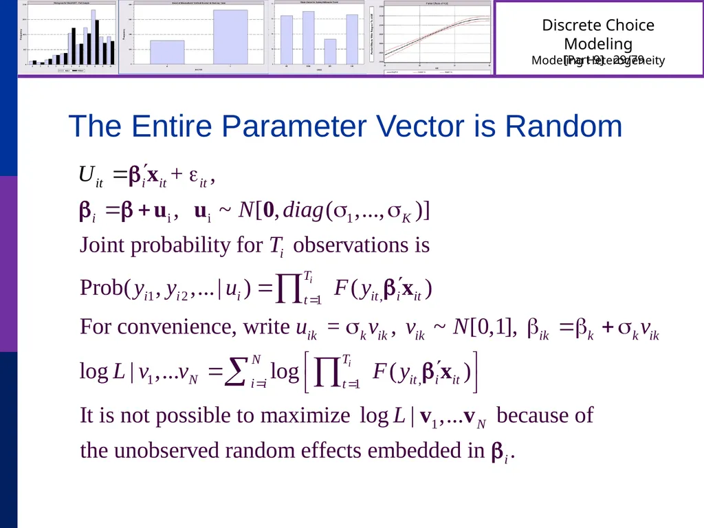
The Entire Parameter Vector is Random<br>
27
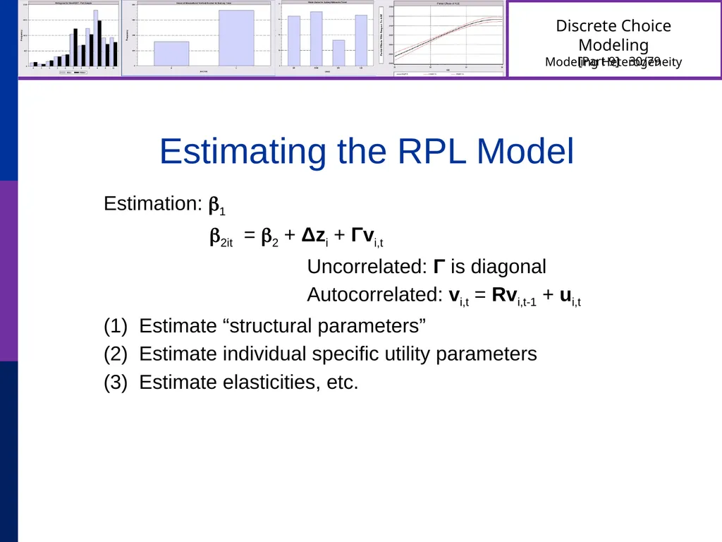
Estimating the RPL Model Estimation: 1
2it = 2 + Δzi + Γvi,t
Uncorrelated: Γ is diagonal
Autocorrelated: vi,t = Rvi,t-1 + ui,t
(1) Estimate “structural parameters”
(2) Estimate individual specific utility parameters
(3) Estimate elasticities, etc.<br>
2it = 2 + Δzi + Γvi,t
Uncorrelated: Γ is diagonal
Autocorrelated: vi,t = Rvi,t-1 + ui,t
(1) Estimate “structural parameters”
(2) Estimate individual specific utility parameters
(3) Estimate elasticities, etc.<br>
28
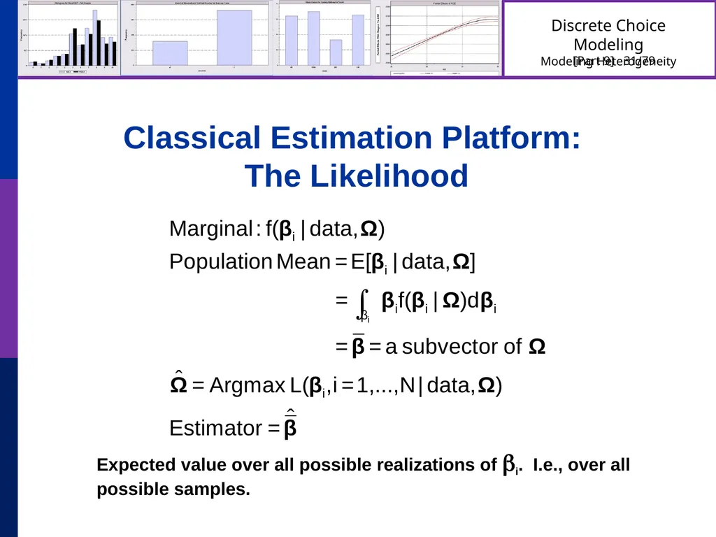
Classical Estimation Platform:
The Likelihood Expected value over all possible realizations of i. I.e., over all possible samples.<br>
29
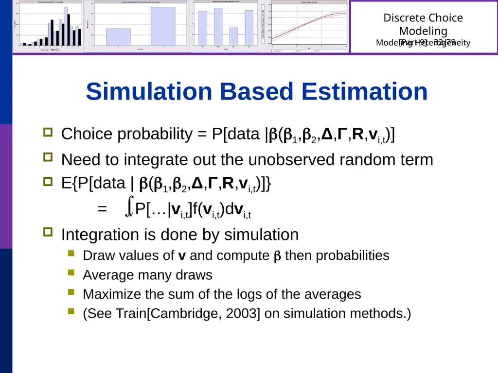
Simulation Based Estimation Choice probability = P[data |(1,2,Δ,Γ,R,vi,t)]
Need to integrate out the unobserved random term
E{P[data | (1,2,Δ,Γ,R,vi,t)]}
= P[…|vi,t]f(vi,t)dvi,t
Integration is done by simulation
Draw values of v and compute then probabilities
Average many draws
Maximize the sum of the logs of the averages
(See Train[Cambridge, 2003] on simulation methods.)<br>
Need to integrate out the unobserved random term
E{P[data | (1,2,Δ,Γ,R,vi,t)]}
= P[…|vi,t]f(vi,t)dvi,t
Integration is done by simulation
Draw values of v and compute then probabilities
Average many draws
Maximize the sum of the logs of the averages
(See Train[Cambridge, 2003] on simulation methods.)<br>
30
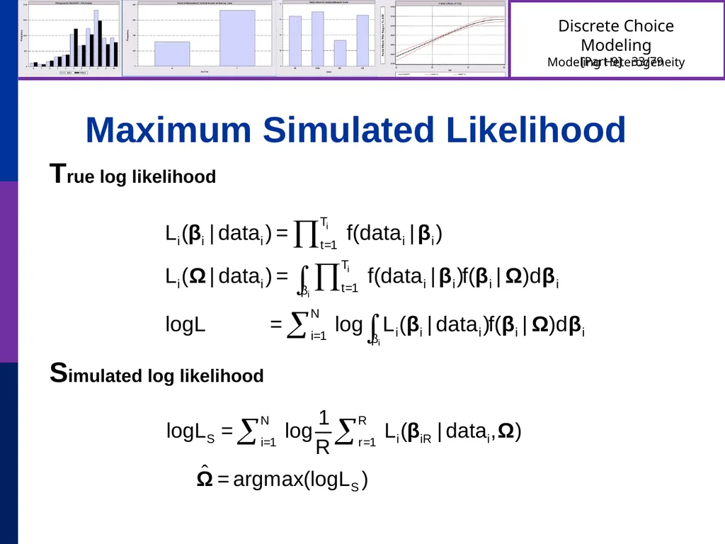
Maximum Simulated Likelihood True log likelihood Simulated log likelihood<br>
31
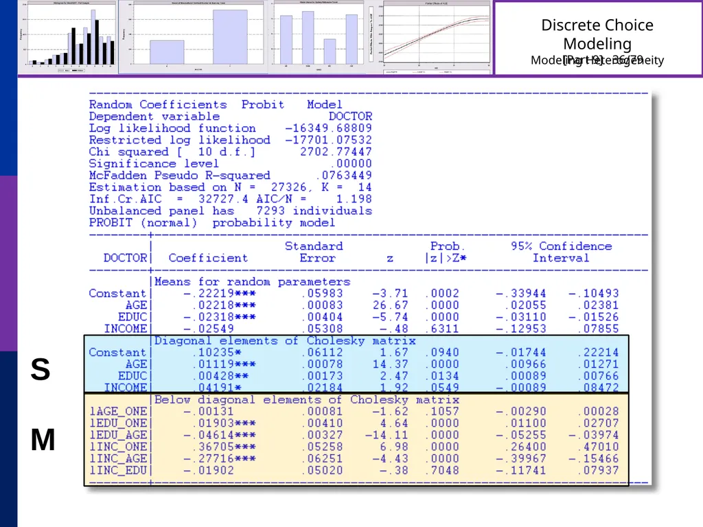
S M<br>
32
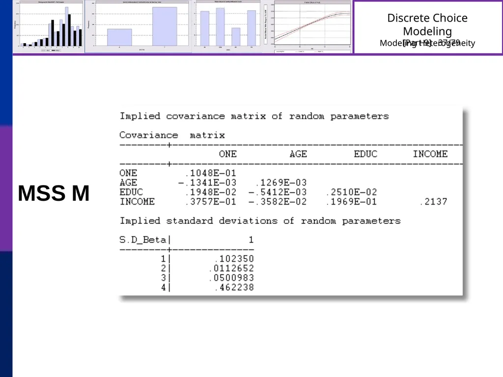
MSSM<br>
33
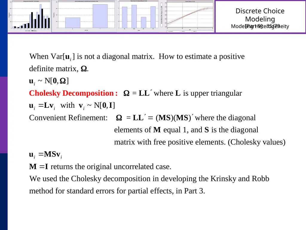
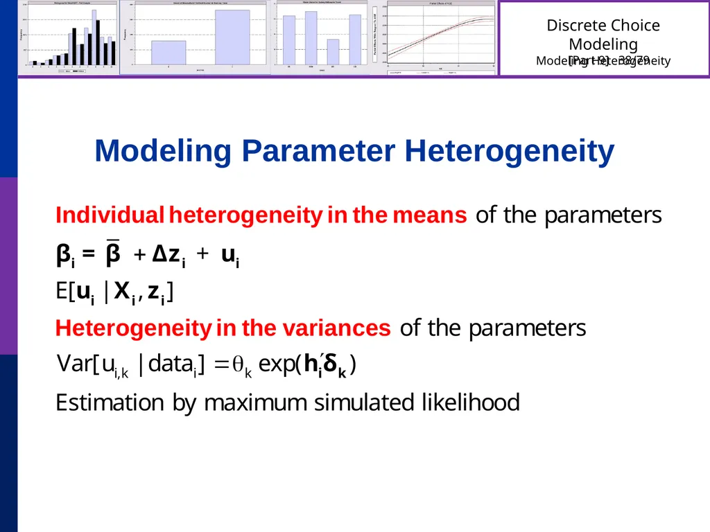
Modeling Parameter Heterogeneity<br>
34
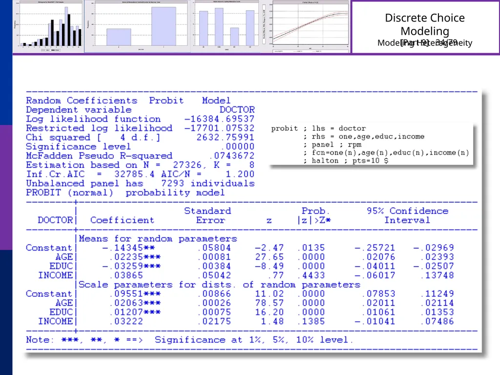
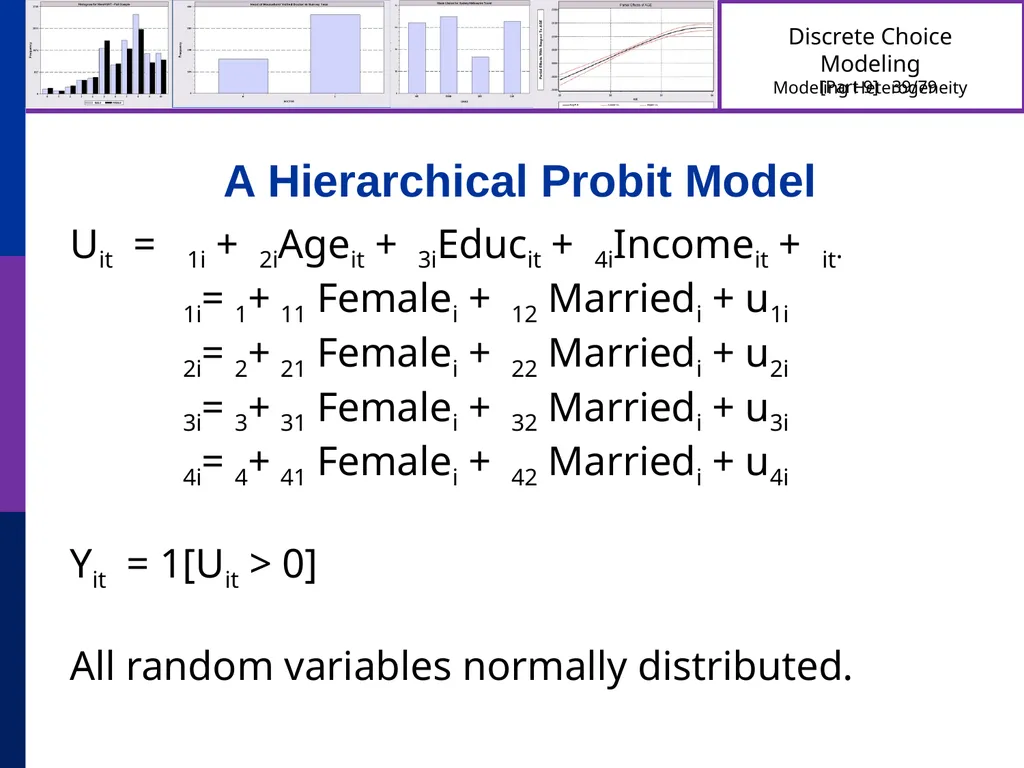
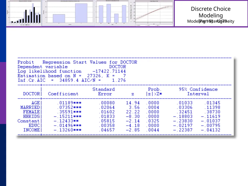
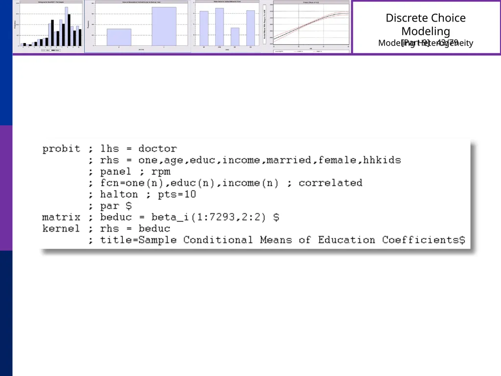
A Hierarchical Probit Model Uit = 1i + 2iAgeit + 3iEducit + 4iIncomeit + it.
1i=1+11 Femalei + 12 Marriedi + u1i
2i=2+21 Femalei + 22 Marriedi + u2i
3i=3+31 Femalei + 32 Marriedi + u3i
4i=4+41 Femalei + 42 Marriedi + u4i
Yit = 1[Uit > 0]
All random variables normally distributed.<br>
1i=1+11 Femalei + 12 Marriedi + u1i
2i=2+21 Femalei + 22 Marriedi + u2i
3i=3+31 Femalei + 32 Marriedi + u3i
4i=4+41 Femalei + 42 Marriedi + u4i
Yit = 1[Uit > 0]
All random variables normally distributed.<br>
35
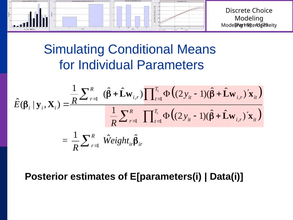
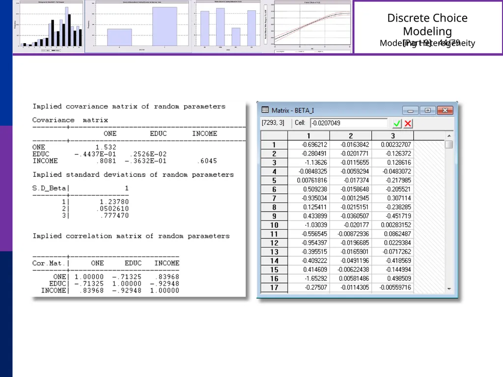
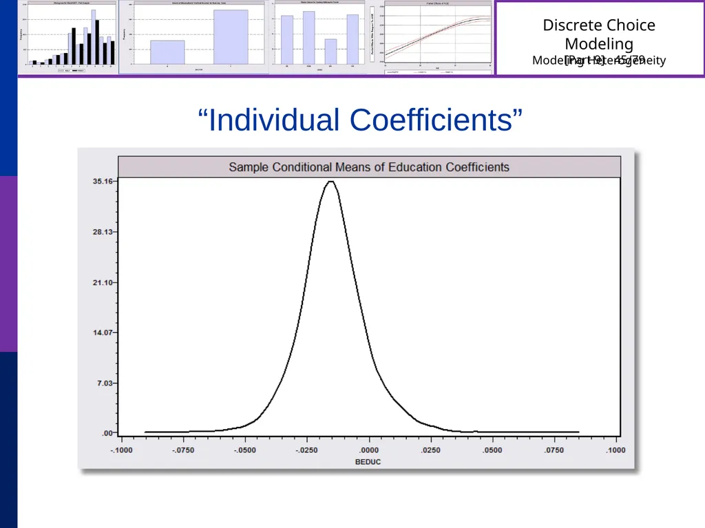
Simulating Conditional Means
for Individual Parameters Posterior estimates of E[parameters(i) | Data(i)]<br>
36
“Individual Coefficients”<br>
37
WinBUGS:
MCMC
User specifies the model – constructs the Gibbs Sampler/Metropolis Hastings
MLWin:
Linear and some nonlinear – logit, Poisson, etc.
Uses MCMC for MLE (noninformative priors)
SAS: Proc Mixed.
Classical
Uses primarily a kind of GLS/GMM (method of moments algorithm for loglinear models)
Stata: Classical
Several loglinear models – GLAMM. Mixing done by quadrature.
Maximum simulated likelihood for multinomial choice (Arne Hole, user provided)
LIMDEP/NLOGIT
Classical
Mixing done by Monte Carlo integration – maximum simulated likelihood
Numerous linear, nonlinear, loglinear models
Ken Train’s Gauss Code, miscellaneous freelance R and Matlab code
Monte Carlo integration
Mixed Logit (mixed multinomial logit) model only (but free!)
Biogeme
Multinomial choice models
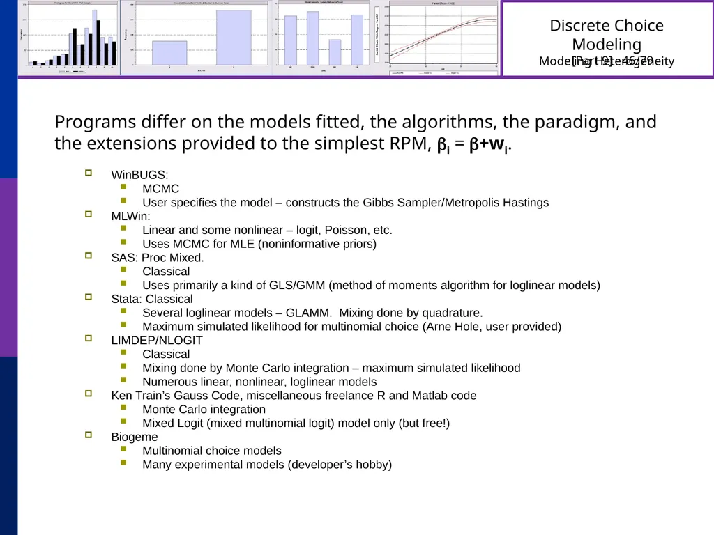
Many experimental models (developer’s hobby) Programs differ on the models fitted, the algorithms, the paradigm, and the extensions provided to the simplest RPM, i = +wi.<br>
MCMC
User specifies the model – constructs the Gibbs Sampler/Metropolis Hastings
MLWin:
Linear and some nonlinear – logit, Poisson, etc.
Uses MCMC for MLE (noninformative priors)
SAS: Proc Mixed.
Classical
Uses primarily a kind of GLS/GMM (method of moments algorithm for loglinear models)
Stata: Classical
Several loglinear models – GLAMM. Mixing done by quadrature.
Maximum simulated likelihood for multinomial choice (Arne Hole, user provided)
LIMDEP/NLOGIT
Classical
Mixing done by Monte Carlo integration – maximum simulated likelihood
Numerous linear, nonlinear, loglinear models
Ken Train’s Gauss Code, miscellaneous freelance R and Matlab code
Monte Carlo integration
Mixed Logit (mixed multinomial logit) model only (but free!)
Biogeme
Multinomial choice models
Many experimental models (developer’s hobby) Programs differ on the models fitted, the algorithms, the paradigm, and the extensions provided to the simplest RPM, i = +wi.<br>
38
Scaling in Choice Models<br>
39
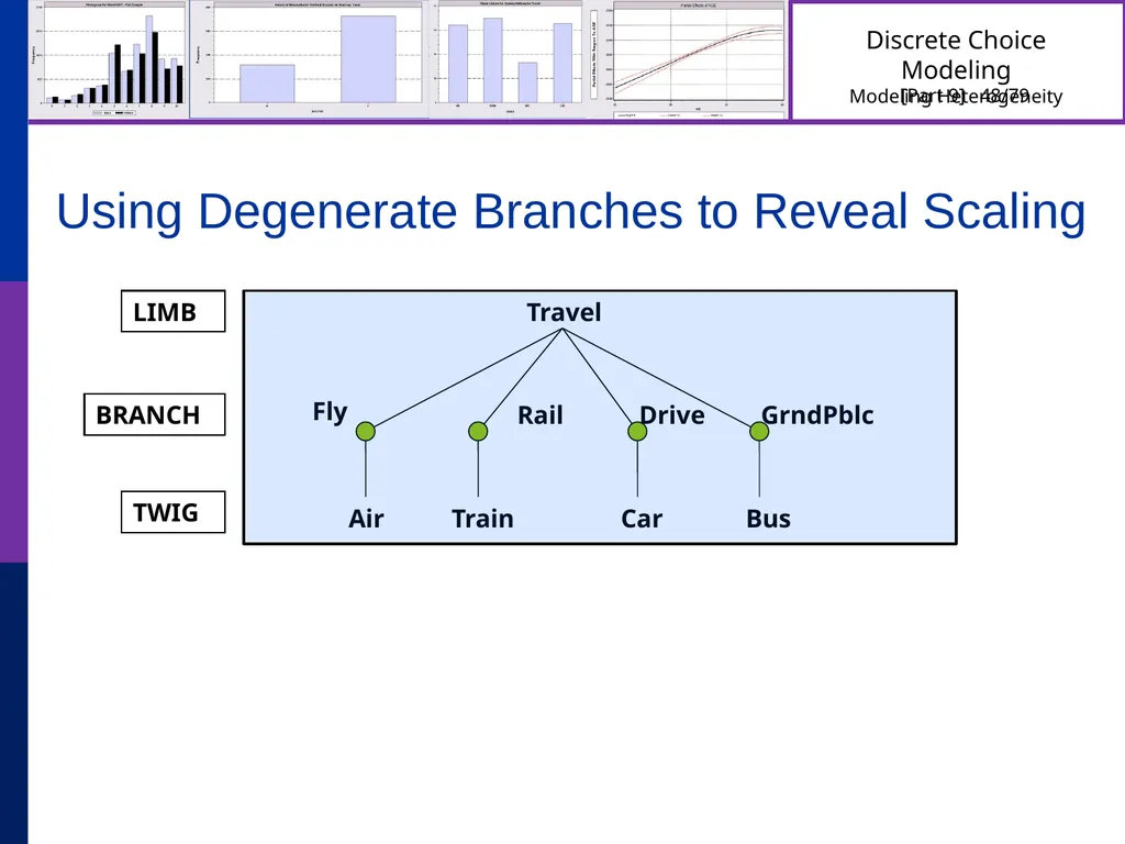
Using Degenerate Branches to Reveal Scaling Travel Fly Rail Air Car Train Bus LIMB BRANCH TWIG Drive GrndPblc<br>
40
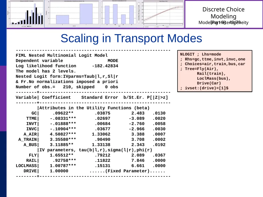
Scaling in Transport Modes -----------------------------------------------------------
FIML Nested Multinomial Logit Model
Dependent variable MODE
Log likelihood function -182.42834
The model has 2 levels.
Nested Logit form:IVparms=Taub|l,r,Sl|r
& Fr.No normalizations imposed a priori
Number of obs.= 210, skipped 0 obs
--------+--------------------------------------------------
Variable| Coefficient Standard Error b/St.Er. P[|Z|>z]
--------+--------------------------------------------------
|Attributes in the Utility Functions (beta)
GC| .09622** .03875 2.483 .0130
TTME| -.08331*** .02697 -3.089 .0020
INVT| -.01888*** .00684 -2.760 .0058
INVC| -.10904*** .03677 -2.966 .0030
A_AIR| 4.50827*** 1.33062 3.388 .0007
A_TRAIN| 3.35580*** .90490 3.708 .0002
A_BUS| 3.11885** 1.33138 2.343 .0192
|IV parameters, tau(b|l,r),sigma(l|r),phi(r)
FLY| 1.65512** .79212 2.089 .0367
RAIL| .92758*** .11822 7.846 .0000
LOCLMASS| 1.00787*** .15131 6.661 .0000
DRIVE| 1.00000 ......(Fixed Parameter)......
--------+-------------------------------------------------- NLOGIT ; Lhs=mode
; Rhs=gc,ttme,invt,invc,one
; Choices=air,train,bus,car
; Tree=Fly(Air), Rail(train),
LoclMass(bus),
Drive(Car)
; ivset:(drive)=[1]$<br>
FIML Nested Multinomial Logit Model
Dependent variable MODE
Log likelihood function -182.42834
The model has 2 levels.
Nested Logit form:IVparms=Taub|l,r,Sl|r
& Fr.No normalizations imposed a priori
Number of obs.= 210, skipped 0 obs
--------+--------------------------------------------------
Variable| Coefficient Standard Error b/St.Er. P[|Z|>z]
--------+--------------------------------------------------
|Attributes in the Utility Functions (beta)
GC| .09622** .03875 2.483 .0130
TTME| -.08331*** .02697 -3.089 .0020
INVT| -.01888*** .00684 -2.760 .0058
INVC| -.10904*** .03677 -2.966 .0030
A_AIR| 4.50827*** 1.33062 3.388 .0007
A_TRAIN| 3.35580*** .90490 3.708 .0002
A_BUS| 3.11885** 1.33138 2.343 .0192
|IV parameters, tau(b|l,r),sigma(l|r),phi(r)
FLY| 1.65512** .79212 2.089 .0367
RAIL| .92758*** .11822 7.846 .0000
LOCLMASS| 1.00787*** .15131 6.661 .0000
DRIVE| 1.00000 ......(Fixed Parameter)......
--------+-------------------------------------------------- NLOGIT ; Lhs=mode
; Rhs=gc,ttme,invt,invc,one
; Choices=air,train,bus,car
; Tree=Fly(Air), Rail(train),
LoclMass(bus),
Drive(Car)
; ivset:(drive)=[1]$<br>
41
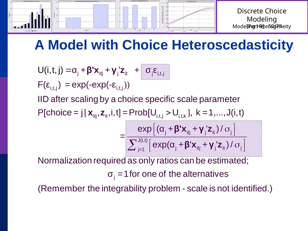
A Model with Choice Heteroscedasticity<br>
42
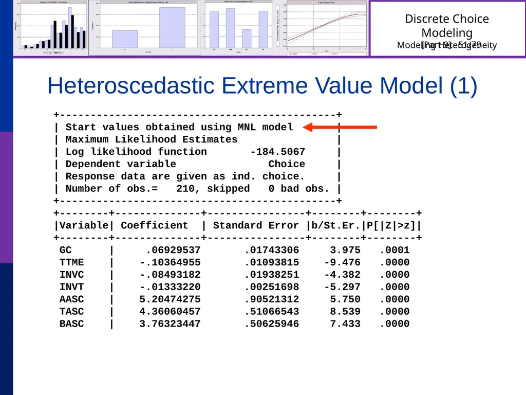
Heteroscedastic Extreme Value Model (1) +---------------------------------------------+
| Start values obtained using MNL model |
| Maximum Likelihood Estimates |
| Log likelihood function -184.5067 |
| Dependent variable Choice |
| Response data are given as ind. choice. |
| Number of obs.= 210, skipped 0 bad obs. |
+---------------------------------------------+
+--------+--------------+----------------+--------+--------+
|Variable| Coefficient | Standard Error |b/St.Er.|P[|Z|>z]|
+--------+--------------+----------------+--------+--------+
GC | .06929537 .01743306 3.975 .0001
TTME | -.10364955 .01093815 -9.476 .0000
INVC | -.08493182 .01938251 -4.382 .0000
INVT | -.01333220 .00251698 -5.297 .0000
AASC | 5.20474275 .90521312 5.750 .0000
TASC | 4.36060457 .51066543 8.539 .0000
BASC | 3.76323447 .50625946 7.433 .0000<br>
| Start values obtained using MNL model |
| Maximum Likelihood Estimates |
| Log likelihood function -184.5067 |
| Dependent variable Choice |
| Response data are given as ind. choice. |
| Number of obs.= 210, skipped 0 bad obs. |
+---------------------------------------------+
+--------+--------------+----------------+--------+--------+
|Variable| Coefficient | Standard Error |b/St.Er.|P[|Z|>z]|
+--------+--------------+----------------+--------+--------+
GC | .06929537 .01743306 3.975 .0001
TTME | -.10364955 .01093815 -9.476 .0000
INVC | -.08493182 .01938251 -4.382 .0000
INVT | -.01333220 .00251698 -5.297 .0000
AASC | 5.20474275 .90521312 5.750 .0000
TASC | 4.36060457 .51066543 8.539 .0000
BASC | 3.76323447 .50625946 7.433 .0000<br>
43
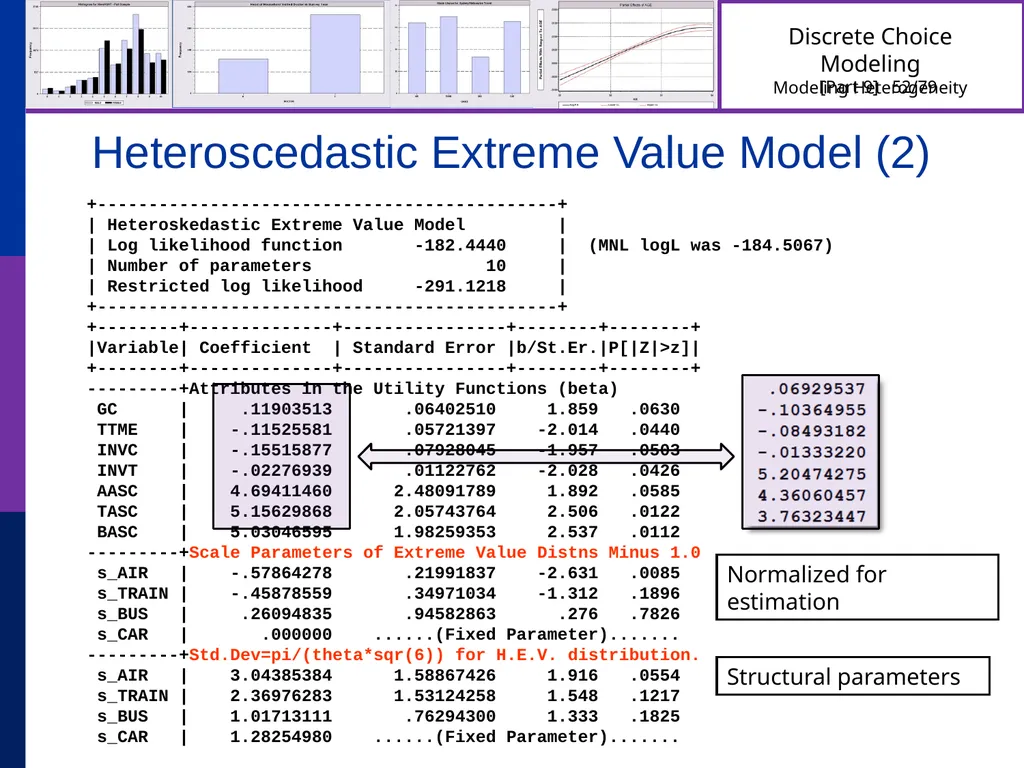
Heteroscedastic Extreme Value Model (2) +---------------------------------------------+
| Heteroskedastic Extreme Value Model |
| Log likelihood function -182.4440 | (MNL logL was -184.5067)
| Number of parameters 10 |
| Restricted log likelihood -291.1218 |
+---------------------------------------------+
+--------+--------------+----------------+--------+--------+
|Variable| Coefficient | Standard Error |b/St.Er.|P[|Z|>z]|
+--------+--------------+----------------+--------+--------+
---------+Attributes in the Utility Functions (beta)
GC | .11903513 .06402510 1.859 .0630
TTME | -.11525581 .05721397 -2.014 .0440
INVC | -.15515877 .07928045 -1.957 .0503
INVT | -.02276939 .01122762 -2.028 .0426
AASC | 4.69411460 2.48091789 1.892 .0585
TASC | 5.15629868 2.05743764 2.506 .0122
BASC | 5.03046595 1.98259353 2.537 .0112
---------+Scale Parameters of Extreme Value Distns Minus 1.0
s_AIR | -.57864278 .21991837 -2.631 .0085
s_TRAIN | -.45878559 .34971034 -1.312 .1896
s_BUS | .26094835 .94582863 .276 .7826
s_CAR | .000000 ......(Fixed Parameter).......
---------+Std.Dev=pi/(theta*sqr(6)) for H.E.V. distribution.
s_AIR | 3.04385384 1.58867426 1.916 .0554
s_TRAIN | 2.36976283 1.53124258 1.548 .1217
s_BUS | 1.01713111 .76294300 1.333 .1825
s_CAR | 1.28254980 ......(Fixed Parameter)....... Normalized for estimation Structural parameters<br>
| Heteroskedastic Extreme Value Model |
| Log likelihood function -182.4440 | (MNL logL was -184.5067)
| Number of parameters 10 |
| Restricted log likelihood -291.1218 |
+---------------------------------------------+
+--------+--------------+----------------+--------+--------+
|Variable| Coefficient | Standard Error |b/St.Er.|P[|Z|>z]|
+--------+--------------+----------------+--------+--------+
---------+Attributes in the Utility Functions (beta)
GC | .11903513 .06402510 1.859 .0630
TTME | -.11525581 .05721397 -2.014 .0440
INVC | -.15515877 .07928045 -1.957 .0503
INVT | -.02276939 .01122762 -2.028 .0426
AASC | 4.69411460 2.48091789 1.892 .0585
TASC | 5.15629868 2.05743764 2.506 .0122
BASC | 5.03046595 1.98259353 2.537 .0112
---------+Scale Parameters of Extreme Value Distns Minus 1.0
s_AIR | -.57864278 .21991837 -2.631 .0085
s_TRAIN | -.45878559 .34971034 -1.312 .1896
s_BUS | .26094835 .94582863 .276 .7826
s_CAR | .000000 ......(Fixed Parameter).......
---------+Std.Dev=pi/(theta*sqr(6)) for H.E.V. distribution.
s_AIR | 3.04385384 1.58867426 1.916 .0554
s_TRAIN | 2.36976283 1.53124258 1.548 .1217
s_BUS | 1.01713111 .76294300 1.333 .1825
s_CAR | 1.28254980 ......(Fixed Parameter)....... Normalized for estimation Structural parameters<br>
44
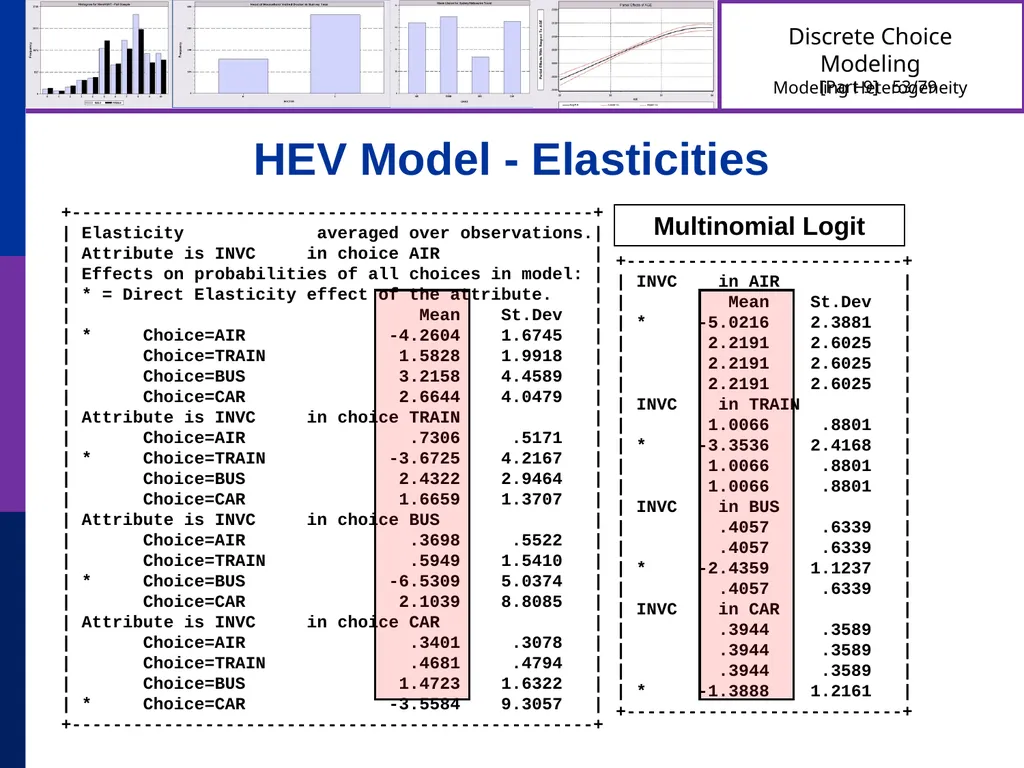
HEV Model - Elasticities +---------------------------------------------------+
| Elasticity averaged over observations.|
| Attribute is INVC in choice AIR |
| Effects on probabilities of all choices in model: |
| * = Direct Elasticity effect of the attribute. |
| Mean St.Dev |
| * Choice=AIR -4.2604 1.6745 |
| Choice=TRAIN 1.5828 1.9918 |
| Choice=BUS 3.2158 4.4589 |
| Choice=CAR 2.6644 4.0479 |
| Attribute is INVC in choice TRAIN |
| Choice=AIR .7306 .5171 |
| * Choice=TRAIN -3.6725 4.2167 |
| Choice=BUS 2.4322 2.9464 |
| Choice=CAR 1.6659 1.3707 |
| Attribute is INVC in choice BUS |
| Choice=AIR .3698 .5522 |
| Choice=TRAIN .5949 1.5410 |
| * Choice=BUS -6.5309 5.0374 |
| Choice=CAR 2.1039 8.8085 |
| Attribute is INVC in choice CAR |
| Choice=AIR .3401 .3078 |
| Choice=TRAIN .4681 .4794 |
| Choice=BUS 1.4723 1.6322 |
| * Choice=CAR -3.5584 9.3057 |
+---------------------------------------------------+ +---------------------------+
| INVC in AIR |
| Mean St.Dev |
| * -5.0216 2.3881 |
| 2.2191 2.6025 |
| 2.2191 2.6025 |
| 2.2191 2.6025 |
| INVC in TRAIN |
| 1.0066 .8801 |
| * -3.3536 2.4168 |
| 1.0066 .8801 |
| 1.0066 .8801 |
| INVC in BUS |
| .4057 .6339 |
| .4057 .6339 |
| * -2.4359 1.1237 |
| .4057 .6339 |
| INVC in CAR |
| .3944 .3589 |
| .3944 .3589 |
| .3944 .3589 |
| * -1.3888 1.2161 |
+---------------------------+ Multinomial Logit<br>
| Elasticity averaged over observations.|
| Attribute is INVC in choice AIR |
| Effects on probabilities of all choices in model: |
| * = Direct Elasticity effect of the attribute. |
| Mean St.Dev |
| * Choice=AIR -4.2604 1.6745 |
| Choice=TRAIN 1.5828 1.9918 |
| Choice=BUS 3.2158 4.4589 |
| Choice=CAR 2.6644 4.0479 |
| Attribute is INVC in choice TRAIN |
| Choice=AIR .7306 .5171 |
| * Choice=TRAIN -3.6725 4.2167 |
| Choice=BUS 2.4322 2.9464 |
| Choice=CAR 1.6659 1.3707 |
| Attribute is INVC in choice BUS |
| Choice=AIR .3698 .5522 |
| Choice=TRAIN .5949 1.5410 |
| * Choice=BUS -6.5309 5.0374 |
| Choice=CAR 2.1039 8.8085 |
| Attribute is INVC in choice CAR |
| Choice=AIR .3401 .3078 |
| Choice=TRAIN .4681 .4794 |
| Choice=BUS 1.4723 1.6322 |
| * Choice=CAR -3.5584 9.3057 |
+---------------------------------------------------+ +---------------------------+
| INVC in AIR |
| Mean St.Dev |
| * -5.0216 2.3881 |
| 2.2191 2.6025 |
| 2.2191 2.6025 |
| 2.2191 2.6025 |
| INVC in TRAIN |
| 1.0066 .8801 |
| * -3.3536 2.4168 |
| 1.0066 .8801 |
| 1.0066 .8801 |
| INVC in BUS |
| .4057 .6339 |
| .4057 .6339 |
| * -2.4359 1.1237 |
| .4057 .6339 |
| INVC in CAR |
| .3944 .3589 |
| .3944 .3589 |
| .3944 .3589 |
| * -1.3888 1.2161 |
+---------------------------+ Multinomial Logit<br>
45
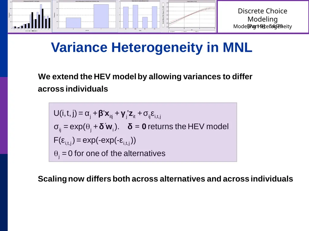
Variance Heterogeneity in MNL<br>
46
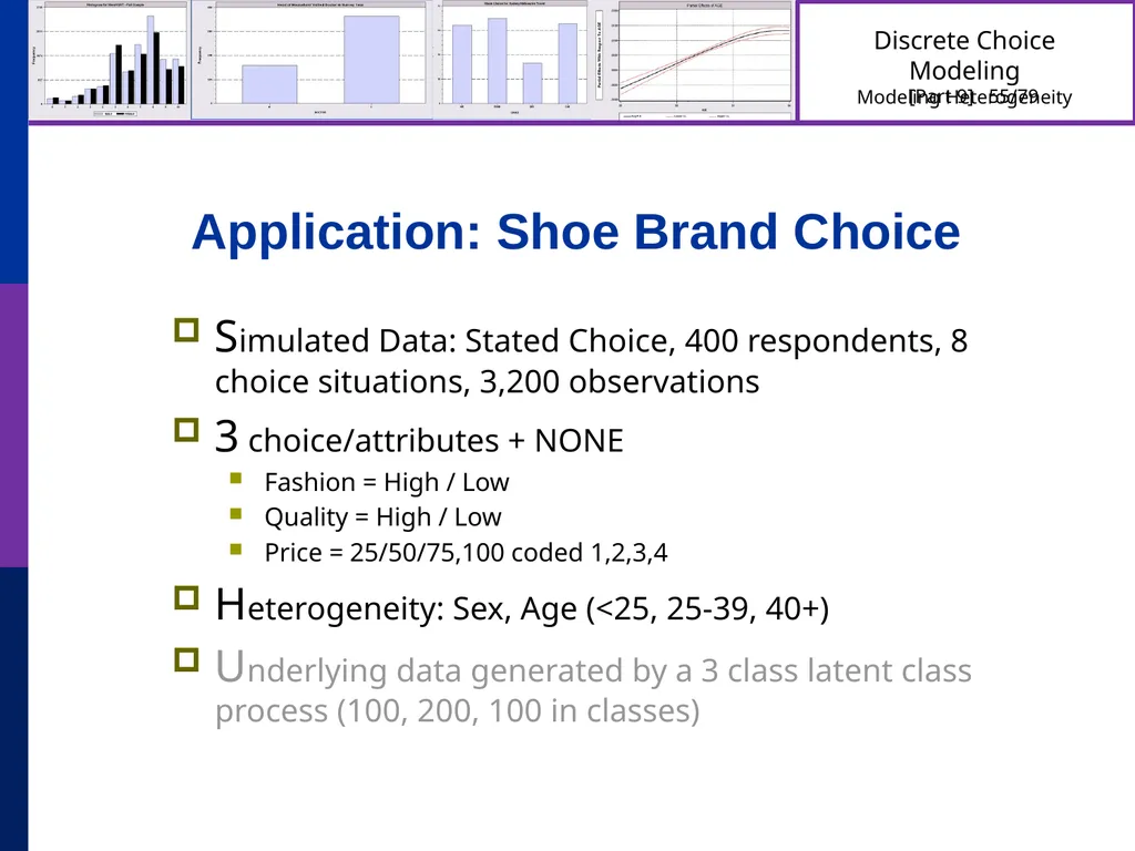
Application: Shoe Brand Choice Simulated Data: Stated Choice, 400 respondents, 8 choice situations, 3,200 observations
3 choice/attributes + NONE
Fashion = High / Low
Quality = High / Low
Price = 25/50/75,100 coded 1,2,3,4
Heterogeneity: Sex, Age (<25, 25-39, 40+)
Underlying data generated by a 3 class latent class process (100, 200, 100 in classes)<br>
3 choice/attributes + NONE
Fashion = High / Low
Quality = High / Low
Price = 25/50/75,100 coded 1,2,3,4
Heterogeneity: Sex, Age (<25, 25-39, 40+)
Underlying data generated by a 3 class latent class process (100, 200, 100 in classes)<br>
47
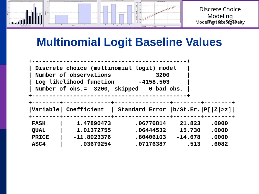
Multinomial Logit Baseline Values +---------------------------------------------+
| Discrete choice (multinomial logit) model |
| Number of observations 3200 |
| Log likelihood function -4158.503 |
| Number of obs.= 3200, skipped 0 bad obs. |
+---------------------------------------------+
+--------+--------------+----------------+--------+--------+
|Variable| Coefficient | Standard Error |b/St.Er.|P[|Z|>z]|
+--------+--------------+----------------+--------+--------+
FASH | 1.47890473 .06776814 21.823 .0000
QUAL | 1.01372755 .06444532 15.730 .0000
PRICE | -11.8023376 .80406103 -14.678 .0000
ASC4 | .03679254 .07176387 .513 .6082<br>
| Discrete choice (multinomial logit) model |
| Number of observations 3200 |
| Log likelihood function -4158.503 |
| Number of obs.= 3200, skipped 0 bad obs. |
+---------------------------------------------+
+--------+--------------+----------------+--------+--------+
|Variable| Coefficient | Standard Error |b/St.Er.|P[|Z|>z]|
+--------+--------------+----------------+--------+--------+
FASH | 1.47890473 .06776814 21.823 .0000
QUAL | 1.01372755 .06444532 15.730 .0000
PRICE | -11.8023376 .80406103 -14.678 .0000
ASC4 | .03679254 .07176387 .513 .6082<br>
48
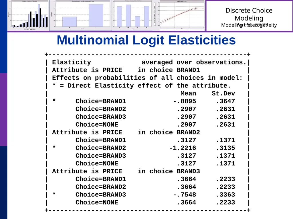
Multinomial Logit Elasticities +---------------------------------------------------+
| Elasticity averaged over observations.|
| Attribute is PRICE in choice BRAND1 |
| Effects on probabilities of all choices in model: |
| * = Direct Elasticity effect of the attribute. |
| Mean St.Dev |
| * Choice=BRAND1 -.8895 .3647 |
| Choice=BRAND2 .2907 .2631 |
| Choice=BRAND3 .2907 .2631 |
| Choice=NONE .2907 .2631 |
| Attribute is PRICE in choice BRAND2 |
| Choice=BRAND1 .3127 .1371 |
| * Choice=BRAND2 -1.2216 .3135 |
| Choice=BRAND3 .3127 .1371 |
| Choice=NONE .3127 .1371 |
| Attribute is PRICE in choice BRAND3 |
| Choice=BRAND1 .3664 .2233 |
| Choice=BRAND2 .3664 .2233 |
| * Choice=BRAND3 -.7548 .3363 |
| Choice=NONE .3664 .2233 |
+---------------------------------------------------+<br>
| Elasticity averaged over observations.|
| Attribute is PRICE in choice BRAND1 |
| Effects on probabilities of all choices in model: |
| * = Direct Elasticity effect of the attribute. |
| Mean St.Dev |
| * Choice=BRAND1 -.8895 .3647 |
| Choice=BRAND2 .2907 .2631 |
| Choice=BRAND3 .2907 .2631 |
| Choice=NONE .2907 .2631 |
| Attribute is PRICE in choice BRAND2 |
| Choice=BRAND1 .3127 .1371 |
| * Choice=BRAND2 -1.2216 .3135 |
| Choice=BRAND3 .3127 .1371 |
| Choice=NONE .3127 .1371 |
| Attribute is PRICE in choice BRAND3 |
| Choice=BRAND1 .3664 .2233 |
| Choice=BRAND2 .3664 .2233 |
| * Choice=BRAND3 -.7548 .3363 |
| Choice=NONE .3664 .2233 |
+---------------------------------------------------+<br>
49
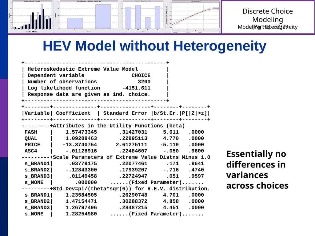
HEV Model without Heterogeneity +---------------------------------------------+
| Heteroskedastic Extreme Value Model |
| Dependent variable CHOICE |
| Number of observations 3200 |
| Log likelihood function -4151.611 |
| Response data are given as ind. choice. |
+---------------------------------------------+
+--------+--------------+----------------+--------+--------+
|Variable| Coefficient | Standard Error |b/St.Er.|P[|Z|>z]|
+--------+--------------+----------------+--------+--------+
---------+Attributes in the Utility Functions (beta)
FASH | 1.57473345 .31427031 5.011 .0000
QUAL | 1.09208463 .22895113 4.770 .0000
PRICE | -13.3740754 2.61275111 -5.119 .0000
ASC4 | -.01128916 .22484607 -.050 .9600
---------+Scale Parameters of Extreme Value Distns Minus 1.0
s_BRAND1| .03779175 .22077461 .171 .8641
s_BRAND2| -.12843300 .17939207 -.716 .4740
s_BRAND3| .01149458 .22724947 .051 .9597
s_NONE | .000000 ......(Fixed Parameter).......
---------+Std.Dev=pi/(theta*sqr(6)) for H.E.V. distribution.
s_BRAND1| 1.23584505 .26290748 4.701 .0000
s_BRAND2| 1.47154471 .30288372 4.858 .0000
s_BRAND3| 1.26797496 .28487215 4.451 .0000
s_NONE | 1.28254980 ......(Fixed Parameter)....... Essentially no differences in variances across choices<br>
| Heteroskedastic Extreme Value Model |
| Dependent variable CHOICE |
| Number of observations 3200 |
| Log likelihood function -4151.611 |
| Response data are given as ind. choice. |
+---------------------------------------------+
+--------+--------------+----------------+--------+--------+
|Variable| Coefficient | Standard Error |b/St.Er.|P[|Z|>z]|
+--------+--------------+----------------+--------+--------+
---------+Attributes in the Utility Functions (beta)
FASH | 1.57473345 .31427031 5.011 .0000
QUAL | 1.09208463 .22895113 4.770 .0000
PRICE | -13.3740754 2.61275111 -5.119 .0000
ASC4 | -.01128916 .22484607 -.050 .9600
---------+Scale Parameters of Extreme Value Distns Minus 1.0
s_BRAND1| .03779175 .22077461 .171 .8641
s_BRAND2| -.12843300 .17939207 -.716 .4740
s_BRAND3| .01149458 .22724947 .051 .9597
s_NONE | .000000 ......(Fixed Parameter).......
---------+Std.Dev=pi/(theta*sqr(6)) for H.E.V. distribution.
s_BRAND1| 1.23584505 .26290748 4.701 .0000
s_BRAND2| 1.47154471 .30288372 4.858 .0000
s_BRAND3| 1.26797496 .28487215 4.451 .0000
s_NONE | 1.28254980 ......(Fixed Parameter)....... Essentially no differences in variances across choices<br>
50
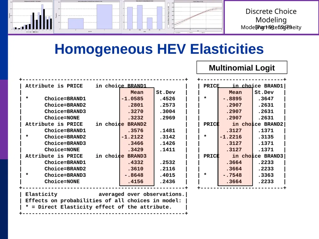
Homogeneous HEV Elasticities +---------------------------------------------------+
| Attribute is PRICE in choice BRAND1 |
| Mean St.Dev |
| * Choice=BRAND1 -1.0585 .4526 |
| Choice=BRAND2 .2801 .2573 |
| Choice=BRAND3 .3270 .3004 |
| Choice=NONE .3232 .2969 |
| Attribute is PRICE in choice BRAND2 |
| Choice=BRAND1 .3576 .1481 |
| * Choice=BRAND2 -1.2122 .3142 |
| Choice=BRAND3 .3466 .1426 |
| Choice=NONE .3429 .1411 |
| Attribute is PRICE in choice BRAND3 |
| Choice=BRAND1 .4332 .2532 |
| Choice=BRAND2 .3610 .2116 |
| * Choice=BRAND3 -.8648 .4015 |
| Choice=NONE .4156 .2436 |
+---------------------------------------------------+
| Elasticity averaged over observations.|
| Effects on probabilities of all choices in model: |
| * = Direct Elasticity effect of the attribute. |
+---------------------------------------------------+ +--------------------------+
| PRICE in choice BRAND1|
| Mean St.Dev |
| * -.8895 .3647 |
| .2907 .2631 |
| .2907 .2631 |
| .2907 .2631 |
| PRICE in choice BRAND2|
| .3127 .1371 |
| * -1.2216 .3135 |
| .3127 .1371 |
| .3127 .1371 |
| PRICE in choice BRAND3|
| .3664 .2233 |
| .3664 .2233 |
| * -.7548 .3363 |
| .3664 .2233 |
+--------------------------+ Multinomial Logit<br>
| Attribute is PRICE in choice BRAND1 |
| Mean St.Dev |
| * Choice=BRAND1 -1.0585 .4526 |
| Choice=BRAND2 .2801 .2573 |
| Choice=BRAND3 .3270 .3004 |
| Choice=NONE .3232 .2969 |
| Attribute is PRICE in choice BRAND2 |
| Choice=BRAND1 .3576 .1481 |
| * Choice=BRAND2 -1.2122 .3142 |
| Choice=BRAND3 .3466 .1426 |
| Choice=NONE .3429 .1411 |
| Attribute is PRICE in choice BRAND3 |
| Choice=BRAND1 .4332 .2532 |
| Choice=BRAND2 .3610 .2116 |
| * Choice=BRAND3 -.8648 .4015 |
| Choice=NONE .4156 .2436 |
+---------------------------------------------------+
| Elasticity averaged over observations.|
| Effects on probabilities of all choices in model: |
| * = Direct Elasticity effect of the attribute. |
+---------------------------------------------------+ +--------------------------+
| PRICE in choice BRAND1|
| Mean St.Dev |
| * -.8895 .3647 |
| .2907 .2631 |
| .2907 .2631 |
| .2907 .2631 |
| PRICE in choice BRAND2|
| .3127 .1371 |
| * -1.2216 .3135 |
| .3127 .1371 |
| .3127 .1371 |
| PRICE in choice BRAND3|
| .3664 .2233 |
| .3664 .2233 |
| * -.7548 .3363 |
| .3664 .2233 |
+--------------------------+ Multinomial Logit<br>
51
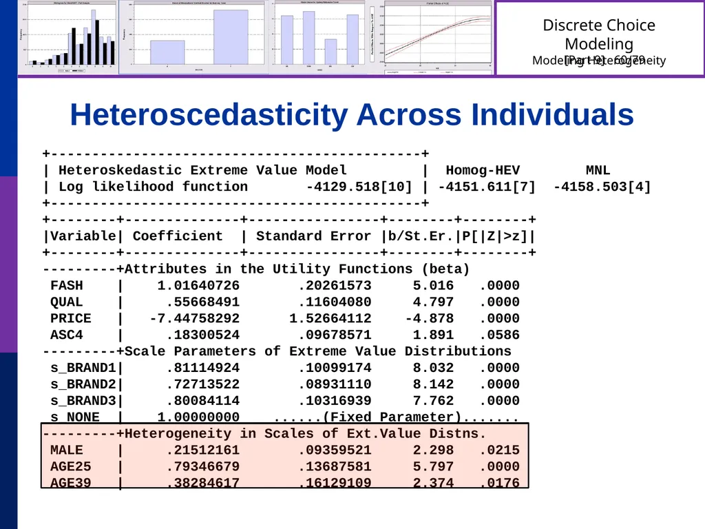
Heteroscedasticity Across Individuals +---------------------------------------------+
| Heteroskedastic Extreme Value Model | Homog-HEV MNL
| Log likelihood function -4129.518[10] | -4151.611[7] -4158.503[4]
+---------------------------------------------+
+--------+--------------+----------------+--------+--------+
|Variable| Coefficient | Standard Error |b/St.Er.|P[|Z|>z]|
+--------+--------------+----------------+--------+--------+
---------+Attributes in the Utility Functions (beta)
FASH | 1.01640726 .20261573 5.016 .0000
QUAL | .55668491 .11604080 4.797 .0000
PRICE | -7.44758292 1.52664112 -4.878 .0000
ASC4 | .18300524 .09678571 1.891 .0586
---------+Scale Parameters of Extreme Value Distributions
s_BRAND1| .81114924 .10099174 8.032 .0000
s_BRAND2| .72713522 .08931110 8.142 .0000
s_BRAND3| .80084114 .10316939 7.762 .0000
s_NONE | 1.00000000 ......(Fixed Parameter).......
---------+Heterogeneity in Scales of Ext.Value Distns.
MALE | .21512161 .09359521 2.298 .0215
AGE25 | .79346679 .13687581 5.797 .0000
AGE39 | .38284617 .16129109 2.374 .0176<br>
| Heteroskedastic Extreme Value Model | Homog-HEV MNL
| Log likelihood function -4129.518[10] | -4151.611[7] -4158.503[4]
+---------------------------------------------+
+--------+--------------+----------------+--------+--------+
|Variable| Coefficient | Standard Error |b/St.Er.|P[|Z|>z]|
+--------+--------------+----------------+--------+--------+
---------+Attributes in the Utility Functions (beta)
FASH | 1.01640726 .20261573 5.016 .0000
QUAL | .55668491 .11604080 4.797 .0000
PRICE | -7.44758292 1.52664112 -4.878 .0000
ASC4 | .18300524 .09678571 1.891 .0586
---------+Scale Parameters of Extreme Value Distributions
s_BRAND1| .81114924 .10099174 8.032 .0000
s_BRAND2| .72713522 .08931110 8.142 .0000
s_BRAND3| .80084114 .10316939 7.762 .0000
s_NONE | 1.00000000 ......(Fixed Parameter).......
---------+Heterogeneity in Scales of Ext.Value Distns.
MALE | .21512161 .09359521 2.298 .0215
AGE25 | .79346679 .13687581 5.797 .0000
AGE39 | .38284617 .16129109 2.374 .0176<br>
52
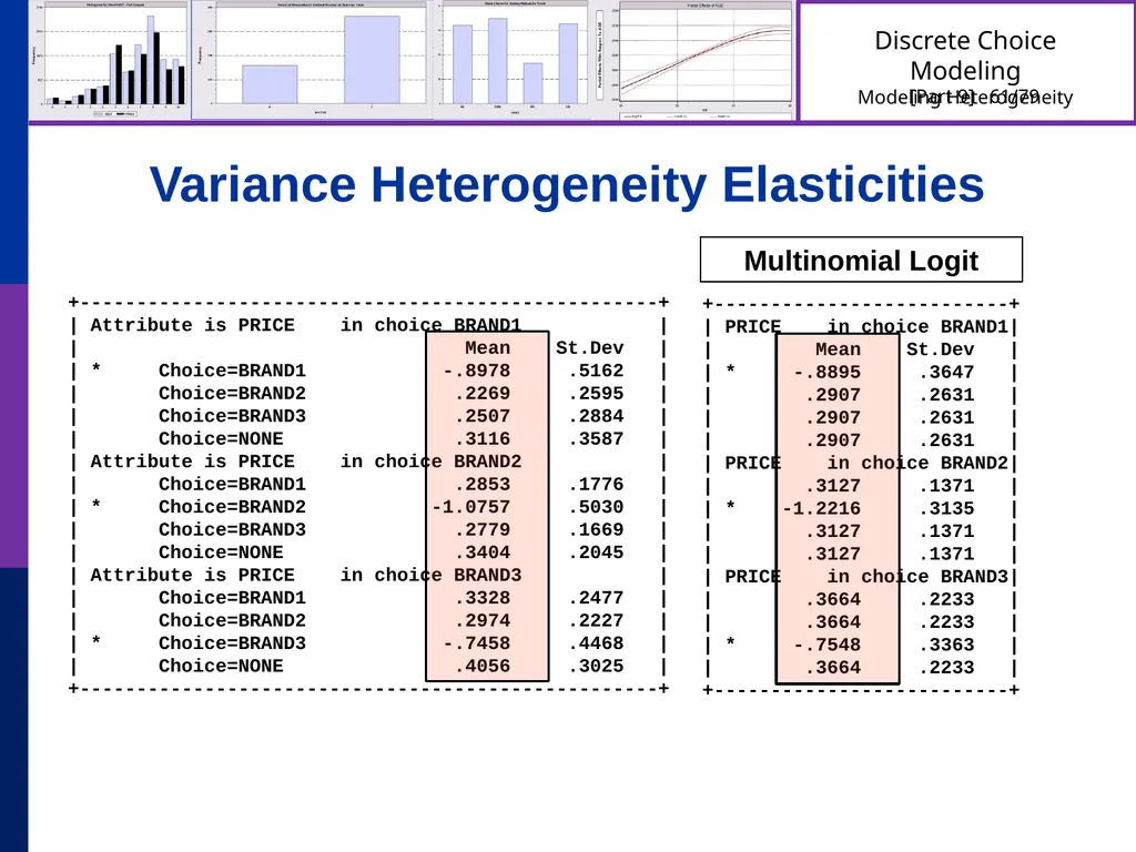
Variance Heterogeneity Elasticities +---------------------------------------------------+
| Attribute is PRICE in choice BRAND1 |
| Mean St.Dev |
| * Choice=BRAND1 -.8978 .5162 |
| Choice=BRAND2 .2269 .2595 |
| Choice=BRAND3 .2507 .2884 |
| Choice=NONE .3116 .3587 |
| Attribute is PRICE in choice BRAND2 |
| Choice=BRAND1 .2853 .1776 |
| * Choice=BRAND2 -1.0757 .5030 |
| Choice=BRAND3 .2779 .1669 |
| Choice=NONE .3404 .2045 |
| Attribute is PRICE in choice BRAND3 |
| Choice=BRAND1 .3328 .2477 |
| Choice=BRAND2 .2974 .2227 |
| * Choice=BRAND3 -.7458 .4468 |
| Choice=NONE .4056 .3025 |
+---------------------------------------------------+ +--------------------------+
| PRICE in choice BRAND1|
| Mean St.Dev |
| * -.8895 .3647 |
| .2907 .2631 |
| .2907 .2631 |
| .2907 .2631 |
| PRICE in choice BRAND2|
| .3127 .1371 |
| * -1.2216 .3135 |
| .3127 .1371 |
| .3127 .1371 |
| PRICE in choice BRAND3|
| .3664 .2233 |
| .3664 .2233 |
| * -.7548 .3363 |
| .3664 .2233 |
+--------------------------+ Multinomial Logit<br>
| Attribute is PRICE in choice BRAND1 |
| Mean St.Dev |
| * Choice=BRAND1 -.8978 .5162 |
| Choice=BRAND2 .2269 .2595 |
| Choice=BRAND3 .2507 .2884 |
| Choice=NONE .3116 .3587 |
| Attribute is PRICE in choice BRAND2 |
| Choice=BRAND1 .2853 .1776 |
| * Choice=BRAND2 -1.0757 .5030 |
| Choice=BRAND3 .2779 .1669 |
| Choice=NONE .3404 .2045 |
| Attribute is PRICE in choice BRAND3 |
| Choice=BRAND1 .3328 .2477 |
| Choice=BRAND2 .2974 .2227 |
| * Choice=BRAND3 -.7458 .4468 |
| Choice=NONE .4056 .3025 |
+---------------------------------------------------+ +--------------------------+
| PRICE in choice BRAND1|
| Mean St.Dev |
| * -.8895 .3647 |
| .2907 .2631 |
| .2907 .2631 |
| .2907 .2631 |
| PRICE in choice BRAND2|
| .3127 .1371 |
| * -1.2216 .3135 |
| .3127 .1371 |
| .3127 .1371 |
| PRICE in choice BRAND3|
| .3664 .2233 |
| .3664 .2233 |
| * -.7548 .3363 |
| .3664 .2233 |
+--------------------------+ Multinomial Logit<br>
53
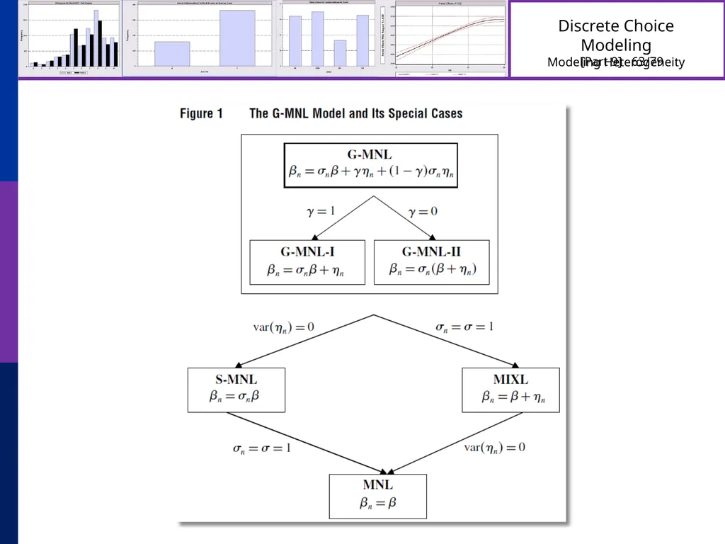
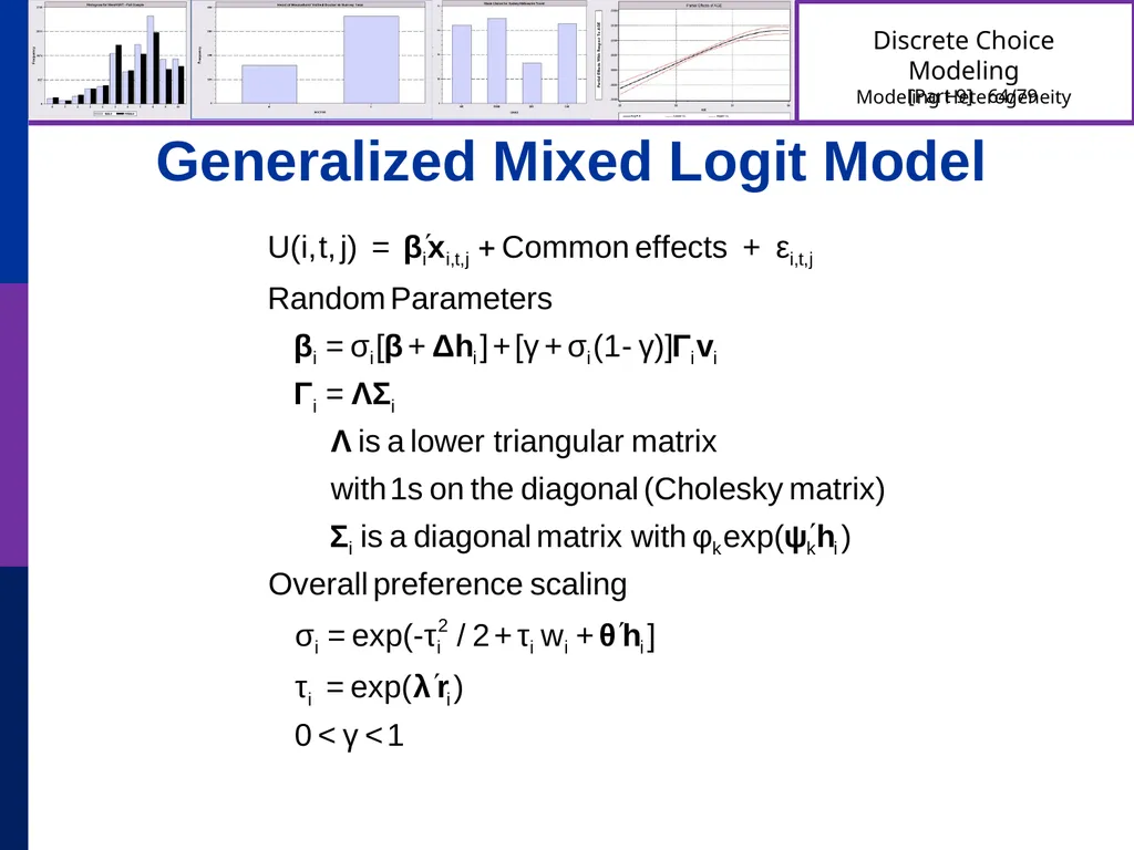
Generalized Mixed Logit Model<br>
54
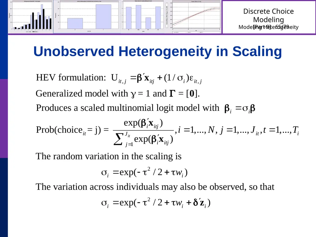
Unobserved Heterogeneity in Scaling<br>
55
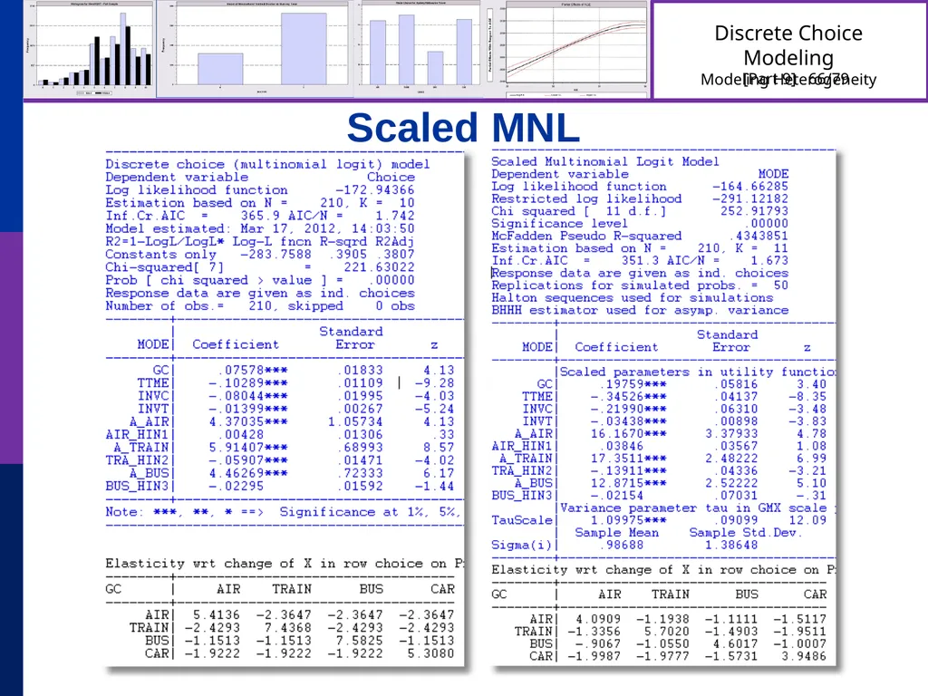
Scaled MNL<br>
56
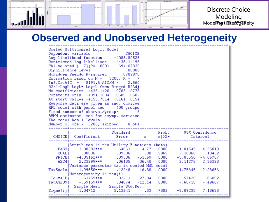
Observed and Unobserved Heterogeneity<br>
57
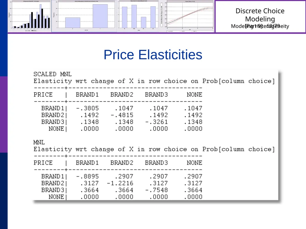
Price Elasticities<br>
58
Scaling as Unobserved Heterogeneity<br>
59
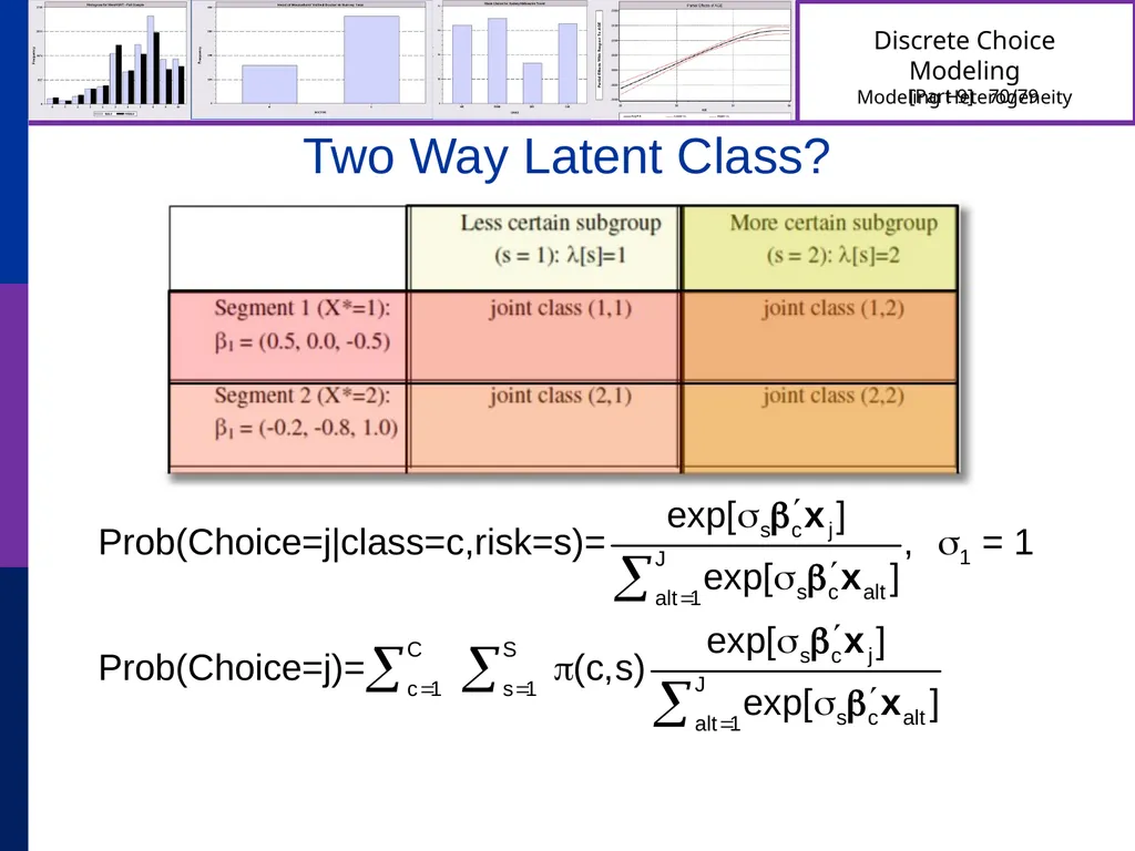
Two Way Latent Class?<br>
60
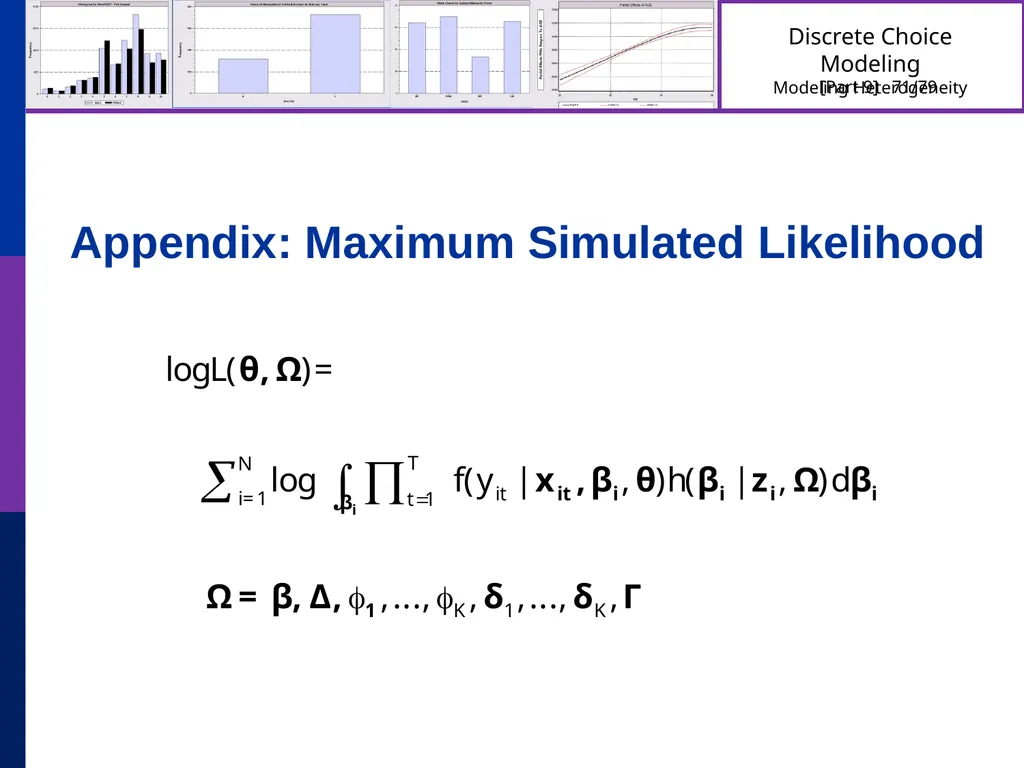
Appendix: Maximum Simulated Likelihood<br>
61
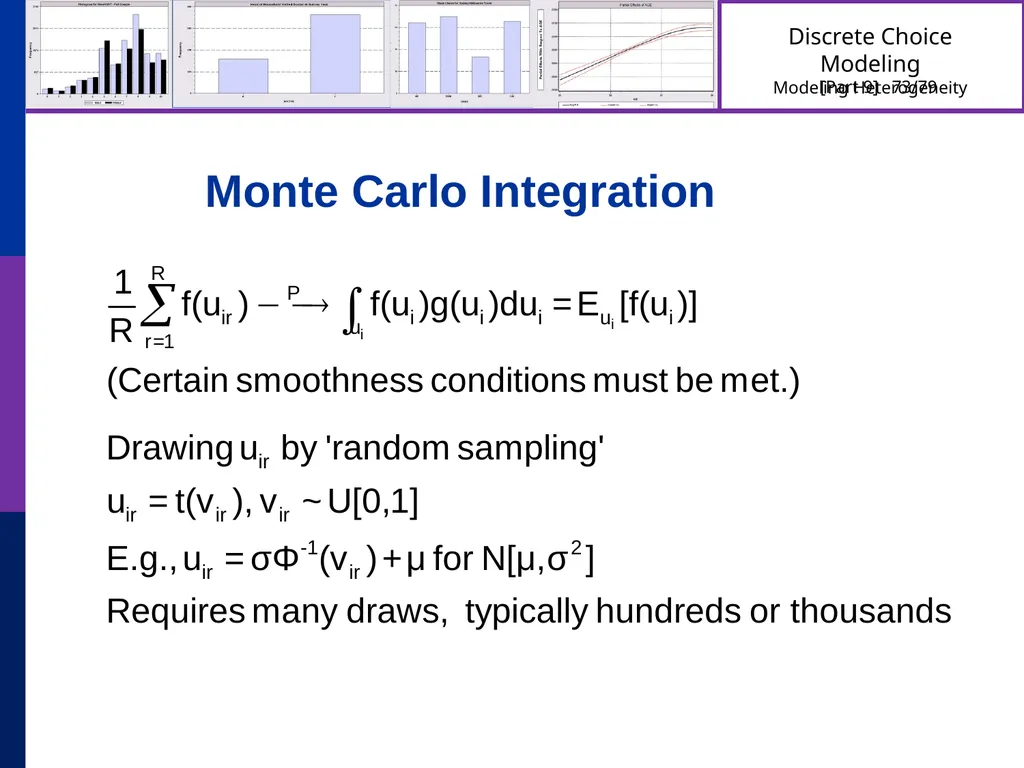
Monte Carlo Integration<br>
62
Monte Carlo Integration<br>
63
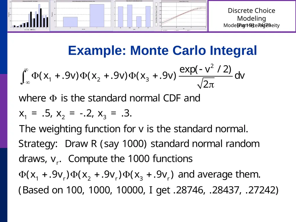
Example: Monte Carlo Integral<br>
64
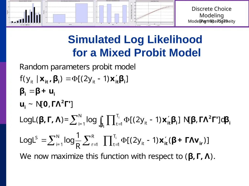
Simulated Log Likelihood
for a Mixed Probit Model<br>
65
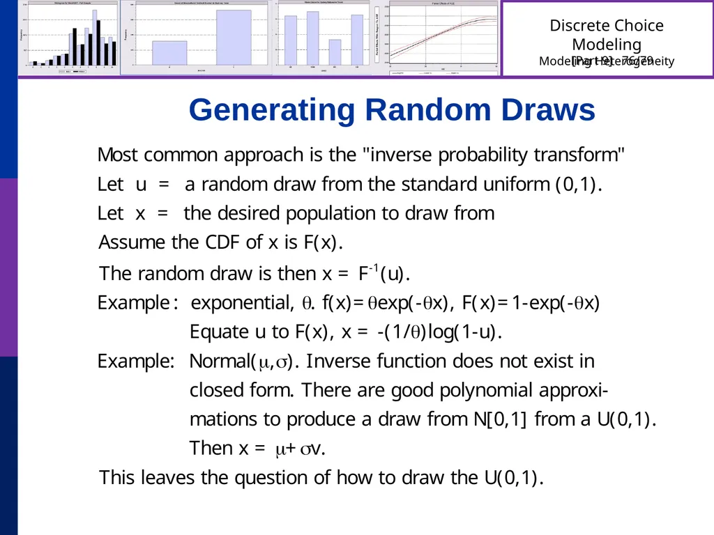
Generating Random Draws<br>
66
Drawing Uniform Random Numbers<br>
67
Quasi-Monte Carlo Integration Based on Halton Sequences For example, using base p=5, the integer r=37 has b0 = 2, b1 = 2, and b2 = 1; (37=1x52 + 2x51 + 2x50). Then
H(37|5) = 25-1 + 25-2 + 15-3 = 0.448.<br>
H(37|5) = 25-1 + 25-2 + 15-3 = 0.448.<br>
68
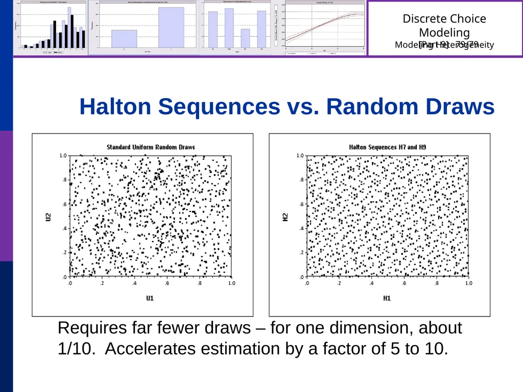
Halton Sequences vs. Random Draws Requires far fewer draws – for one dimension, about 1/10. Accelerates estimation by a factor of 5 to 10.<br>