
Dynamic Flight Simulation (DFS) for MAD/MUTT Erich
YM
Published · 34 slides · 0 views
1 / 1


Description
Dynamic Flight Simulation (DFS) for MADMUTT Erich Ritz and P. C. Chen 9489 E. Ironwood Square Drive, Scottsdale, AZ 85258, Tel. (480) 945-9988, Fax (480) 945-6588, E-mail: infozonatech.com Presented at ASE Workshop, NASA Langley, VA on
Related Topics
Share
Embed code
Download this presentation From Below
"Dynamic Flight Simulation (DFS) for MAD/MUTT Erich" is the property of its rightful owner. Permission is granted to download and print the materials on this website for personal, non-commercial use only, and to display it on your personal computer provided you do not modify the materials and that you retain all copyright notices contained in the materials. By downloading content from our website, you accept the terms of this agreement.
Presentation Transcript
01
Dynamic Flight Simulation (DFS) for MAD/MUTT Erich Ritz and P. C. Chen 9489 E. Ironwood Square Drive, Scottsdale, AZ 85258, Tel. (480) 945-9988, Fax (480) 945-6588, E-mail: info@zonatech.com Presented at ASE Workshop, NASA Langley, VA on April 18-19, 2012<br>
02
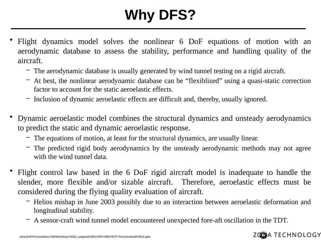
Why DFS? Flight dynamics model solves the nonlinear 6 DoF equations of motion with an aerodynamic database to assess the stability, performance and handling quality of the aircraft.
The aerodynamic database is usually generated by wind tunnel testing on a rigid aircraft.
At best, the nonlinear aerodynamic database can be “flexiblized” using a quasi-static correction factor to account for the static aeroelastic effects.
Inclusion of dynamic aeroelastic effects are difficult and, thereby, usually ignored. Dynamic aeroelastic model combines the structural dynamics and unsteady aerodynamics to predict the static and dynamic aeroelastic response.
The equations of motion, at least for the structural dynamics, are usually linear.
The predicted rigid body aerodynamics by the unsteady aerodynamic methods may not agree with the wind tunnel data. Flight control law based in the 6 DoF rigid aircraft model is inadequate to handle the slender, more flexible and/or sizable aircraft. Therefore, aeroelastic effects must be considered during the flying quality evaluation of aircraft.
Helios mishap in June 2003 possibly due to an interaction between aeroelastic deformation and longitudinal stability.
A sensor-craft wind tunnel model encountered unexpected fore-aft oscillation in the TDT.<br>
The aerodynamic database is usually generated by wind tunnel testing on a rigid aircraft.
At best, the nonlinear aerodynamic database can be “flexiblized” using a quasi-static correction factor to account for the static aeroelastic effects.
Inclusion of dynamic aeroelastic effects are difficult and, thereby, usually ignored. Dynamic aeroelastic model combines the structural dynamics and unsteady aerodynamics to predict the static and dynamic aeroelastic response.
The equations of motion, at least for the structural dynamics, are usually linear.
The predicted rigid body aerodynamics by the unsteady aerodynamic methods may not agree with the wind tunnel data. Flight control law based in the 6 DoF rigid aircraft model is inadequate to handle the slender, more flexible and/or sizable aircraft. Therefore, aeroelastic effects must be considered during the flying quality evaluation of aircraft.
Helios mishap in June 2003 possibly due to an interaction between aeroelastic deformation and longitudinal stability.
A sensor-craft wind tunnel model encountered unexpected fore-aft oscillation in the TDT.<br>
03
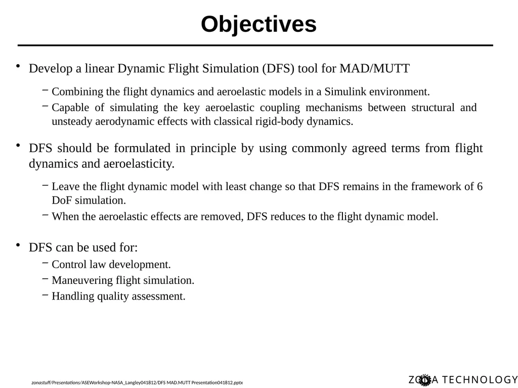
Develop a linear Dynamic Flight Simulation (DFS) tool for MAD/MUTT
Combining the flight dynamics and aeroelastic models in a Simulink environment.
Capable of simulating the key aeroelastic coupling mechanisms between structural and unsteady aerodynamic effects with classical rigid-body dynamics. DFS should be formulated in principle by using commonly agreed terms from flight dynamics and aeroelasticity.
Leave the flight dynamic model with least change so that DFS remains in the framework of 6 DoF simulation.
When the aeroelastic effects are removed, DFS reduces to the flight dynamic model. DFS can be used for:
Control law development.
Maneuvering flight simulation.
Handling quality assessment. Objectives<br>
Combining the flight dynamics and aeroelastic models in a Simulink environment.
Capable of simulating the key aeroelastic coupling mechanisms between structural and unsteady aerodynamic effects with classical rigid-body dynamics. DFS should be formulated in principle by using commonly agreed terms from flight dynamics and aeroelasticity.
Leave the flight dynamic model with least change so that DFS remains in the framework of 6 DoF simulation.
When the aeroelastic effects are removed, DFS reduces to the flight dynamic model. DFS can be used for:
Control law development.
Maneuvering flight simulation.
Handling quality assessment. Objectives<br>
04
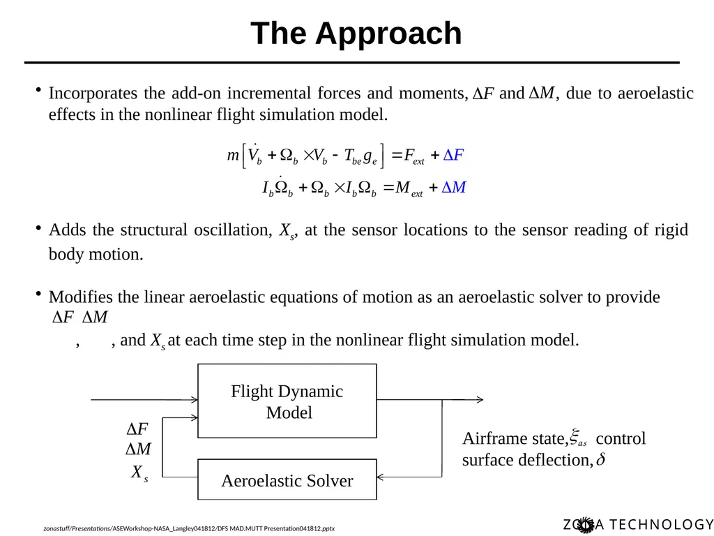
Airframe state, control
surface deflection, The Approach<br>
surface deflection, The Approach<br>
05
Time-Domain Aeroservoelastic
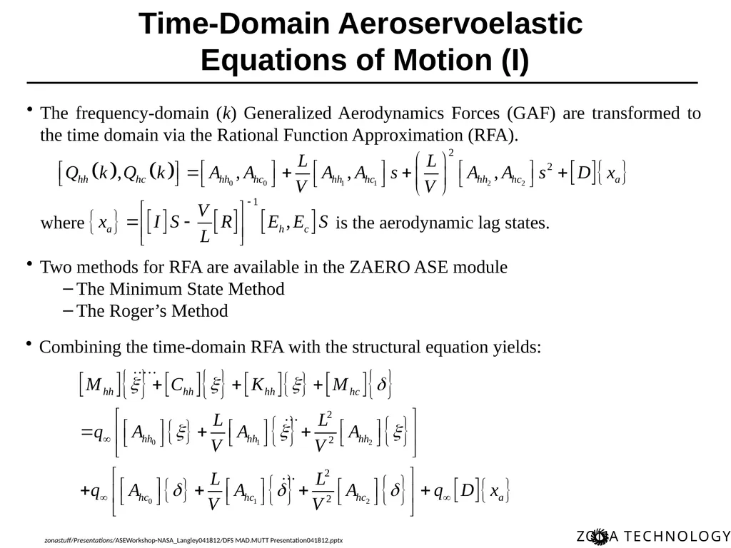
Equations of Motion (I) The frequency-domain (k) Generalized Aerodynamics Forces (GAF) are transformed to the time domain via the Rational Function Approximation (RFA).
where is the aerodynamic lag states. Two methods for RFA are available in the ZAERO ASE module
The Minimum State Method
The Roger’s Method Combining the time-domain RFA with the structural equation yields:<br>
Equations of Motion (I) The frequency-domain (k) Generalized Aerodynamics Forces (GAF) are transformed to the time domain via the Rational Function Approximation (RFA).
where is the aerodynamic lag states. Two methods for RFA are available in the ZAERO ASE module
The Minimum State Method
The Roger’s Method Combining the time-domain RFA with the structural equation yields:<br>
06
Time-Domain Aeroservoelastic
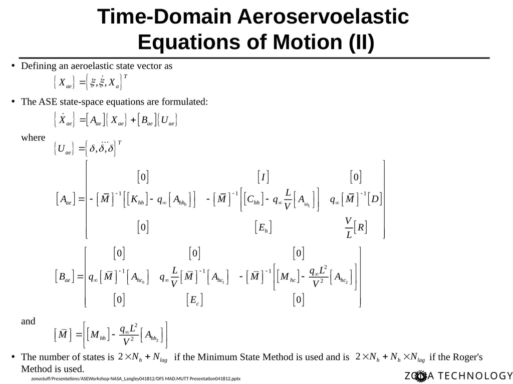
Equations of Motion (II) Defining an aeroelastic state vector as
The ASE state-space equations are formulated:
where
and
The number of states is if the Minimum State Method is used and is if the Roger's Method is used.<br>
Equations of Motion (II) Defining an aeroelastic state vector as
The ASE state-space equations are formulated:
where
and
The number of states is if the Minimum State Method is used and is if the Roger's Method is used.<br>
07
Rigid body modes of the linear aeroelastic equations of motion are usually computed by the finite element analysis and defined in the principle axis.
To be consistent with the flight dynamic model, they must be transformed to the airframe states such as …etc.
The generalized mass matrix of the rigid body modes, usually a diagonal matrix, needs to be converted to the rigid body mass matrix that involves the inertial cross products such as Ixz , Iyz, …, etc. The rigid-body aerodynamics computed by the unsteady aerodynamic methods should be replaced by the wind tunnel data. Gravity should be in the aeroelastic solver.
The linear aeroelastic equations of motion lacks the gravity term.
Without the gravity term, phugoid mode can not be accurately recovered by the aeroelastic solver. If the flight dynamic model is already incorporated with static aeroelastic effects, these effects must be excluded from aeroelastic solver. Technical Issues Involved in the Development
of Aeroelastic Solver<br>
To be consistent with the flight dynamic model, they must be transformed to the airframe states such as …etc.
The generalized mass matrix of the rigid body modes, usually a diagonal matrix, needs to be converted to the rigid body mass matrix that involves the inertial cross products such as Ixz , Iyz, …, etc. The rigid-body aerodynamics computed by the unsteady aerodynamic methods should be replaced by the wind tunnel data. Gravity should be in the aeroelastic solver.
The linear aeroelastic equations of motion lacks the gravity term.
Without the gravity term, phugoid mode can not be accurately recovered by the aeroelastic solver. If the flight dynamic model is already incorporated with static aeroelastic effects, these effects must be excluded from aeroelastic solver. Technical Issues Involved in the Development
of Aeroelastic Solver<br>
08
Transformation of Rigid-Body Modes
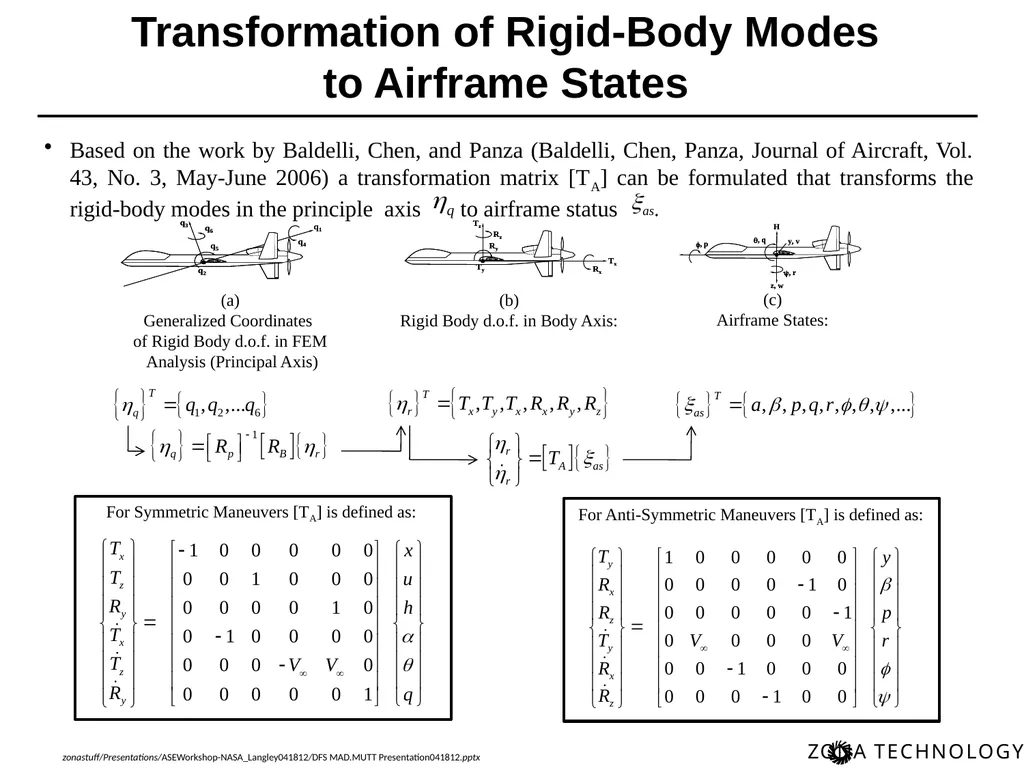
to Airframe States Based on the work by Baldelli, Chen, and Panza (Baldelli, Chen, Panza, Journal of Aircraft, Vol. 43, No. 3, May-June 2006) a transformation matrix [TA] can be formulated that transforms the rigid-body modes in the principle axis to airframe status . For Symmetric Maneuvers [TA] is defined as: For Anti-Symmetric Maneuvers [TA] is defined as: (a)
Generalized Coordinates
of Rigid Body d.o.f. in FEM
Analysis (Principal Axis) (b)
Rigid Body d.o.f. in Body Axis: (c)
Airframe States:<br>
to Airframe States Based on the work by Baldelli, Chen, and Panza (Baldelli, Chen, Panza, Journal of Aircraft, Vol. 43, No. 3, May-June 2006) a transformation matrix [TA] can be formulated that transforms the rigid-body modes in the principle axis to airframe status . For Symmetric Maneuvers [TA] is defined as: For Anti-Symmetric Maneuvers [TA] is defined as: (a)
Generalized Coordinates
of Rigid Body d.o.f. in FEM
Analysis (Principal Axis) (b)
Rigid Body d.o.f. in Body Axis: (c)
Airframe States:<br>
09
Conversion of Generalized Mass Matrix to
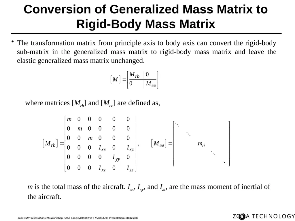
Rigid-Body Mass Matrix where matrices [Mrb] and [Mee] are defined as, m is the total mass of the aircraft. Ixx, Ixy, and Izz, are the mass moment of inertial of the aircraft. The transformation matrix from principle axis to body axis can convert the rigid-body sub-matrix in the generalized mass matrix to rigid-body mass matrix and leave the elastic generalized mass matrix unchanged.<br>
Rigid-Body Mass Matrix where matrices [Mrb] and [Mee] are defined as, m is the total mass of the aircraft. Ixx, Ixy, and Izz, are the mass moment of inertial of the aircraft. The transformation matrix from principle axis to body axis can convert the rigid-body sub-matrix in the generalized mass matrix to rigid-body mass matrix and leave the elastic generalized mass matrix unchanged.<br>
10
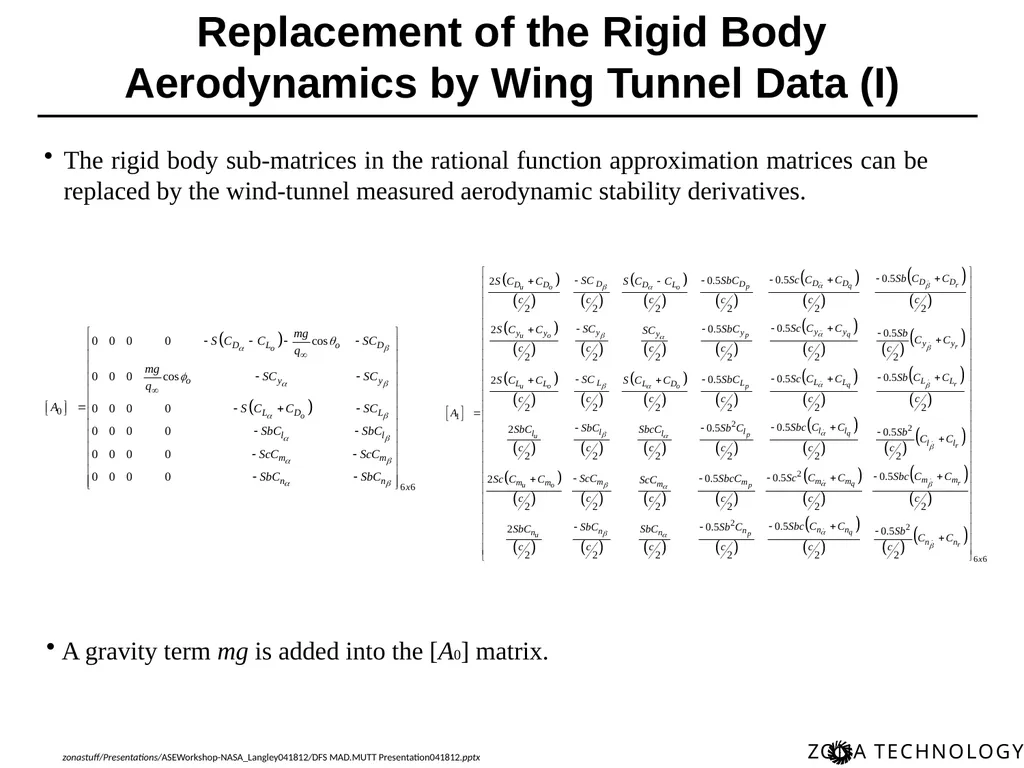
Replacement of the Rigid Body Aerodynamics by Wing Tunnel Data (I) The rigid body sub-matrices in the rational function approximation matrices can be replaced by the wind-tunnel measured aerodynamic stability derivatives. A gravity term mg is added into the [A0] matrix.<br>
11
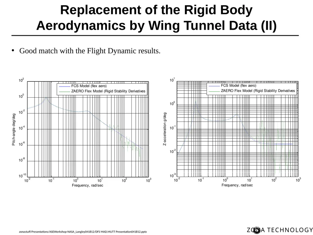
Good match with the Flight Dynamic results. Replacement of the Rigid Body Aerodynamics by Wing Tunnel Data (II)<br>
12
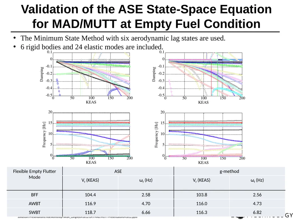
The Minimum State Method with six aerodynamic lag states are used.
6 rigid bodies and 24 elastic modes are included. Validation of the ASE State-Space Equation for MAD/MUTT at Empty Fuel Condition<br>
6 rigid bodies and 24 elastic modes are included. Validation of the ASE State-Space Equation for MAD/MUTT at Empty Fuel Condition<br>
13
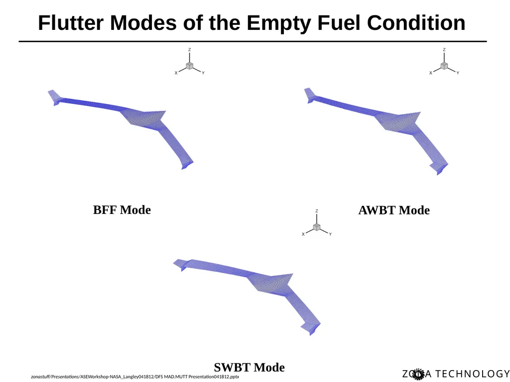
Flutter Modes of the Empty Fuel Condition BFF Mode AWBT Mode SWBT Mode<br>
14
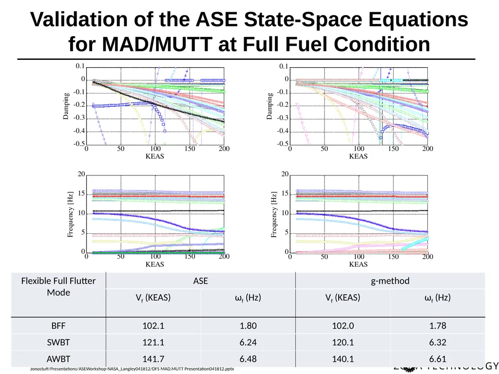
Validation of the ASE State-Space Equations for MAD/MUTT at Full Fuel Condition<br>
15
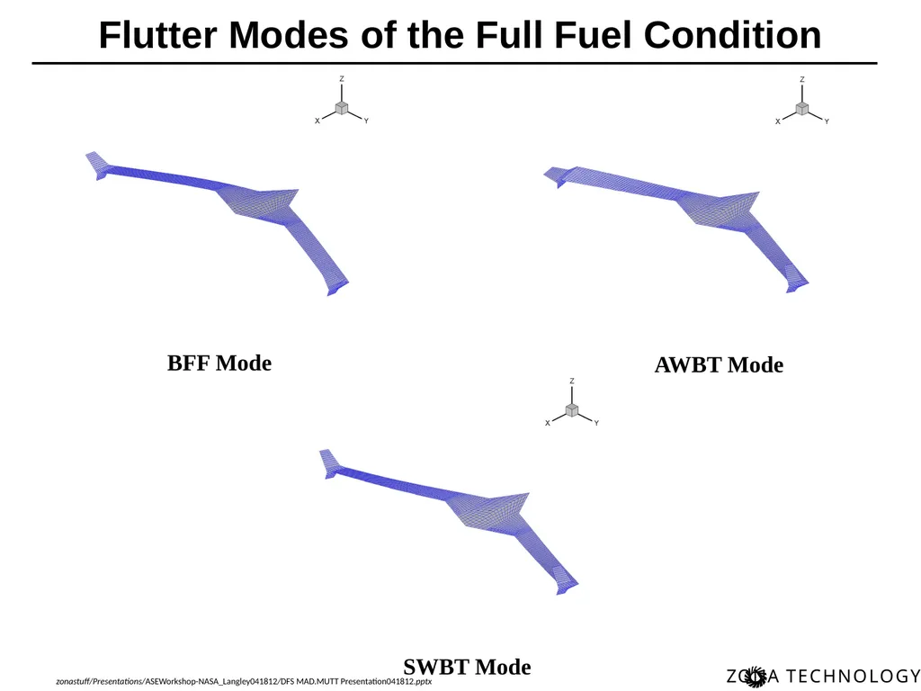
Flutter Modes of the Full Fuel Condition BFF Mode SWBT Mode AWBT Mode<br>
16
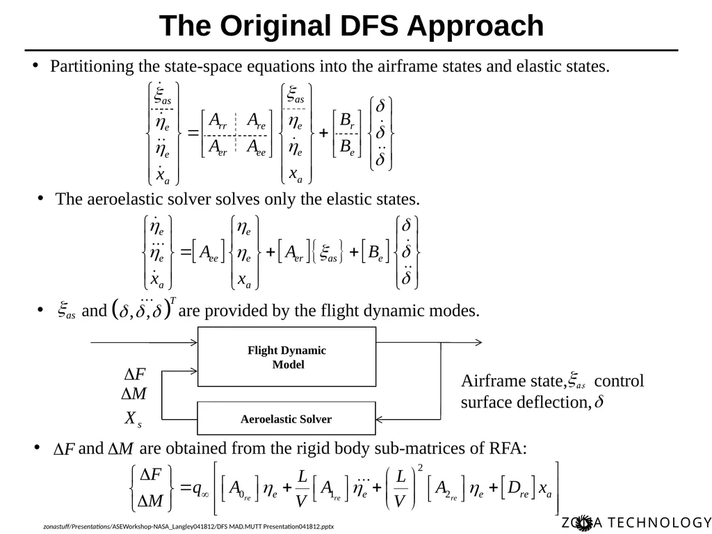
The Original DFS Approach Partitioning the state-space equations into the airframe states and elastic states. The aeroelastic solver solves only the elastic states.<br>
17
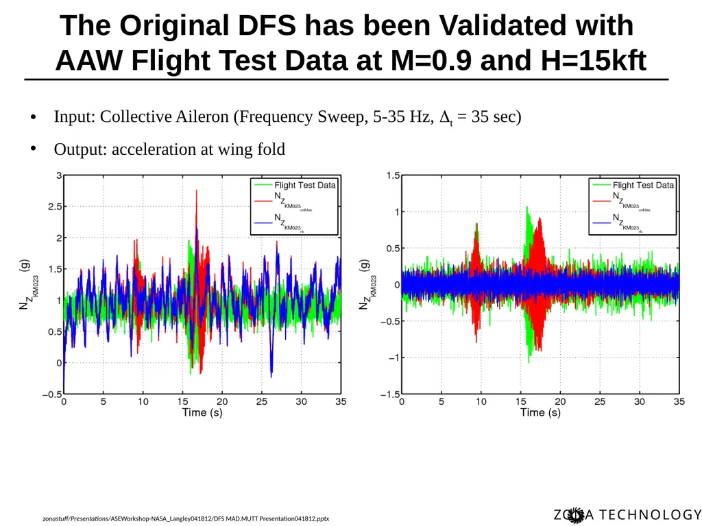
The Original DFS has been Validated with
AAW Flight Test Data at M=0.9 and H=15kft Input: Collective Aileron (Frequency Sweep, 5-35 Hz, t = 35 sec)
Output: acceleration at wing fold<br>
AAW Flight Test Data at M=0.9 and H=15kft Input: Collective Aileron (Frequency Sweep, 5-35 Hz, t = 35 sec)
Output: acceleration at wing fold<br>
18
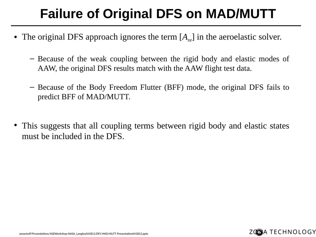
Failure of Original DFS on MAD/MUTT The original DFS approach ignores the term [Are] in the aeroelastic solver.
Because of the weak coupling between the rigid body and elastic modes of AAW, the original DFS results match with the AAW flight test data.
Because of the Body Freedom Flutter (BFF) mode, the original DFS fails to predict BFF of MAD/MUTT.
This suggests that all coupling terms between rigid body and elastic states must be included in the DFS.<br>
Because of the weak coupling between the rigid body and elastic modes of AAW, the original DFS results match with the AAW flight test data.
Because of the Body Freedom Flutter (BFF) mode, the original DFS fails to predict BFF of MAD/MUTT.
This suggests that all coupling terms between rigid body and elastic states must be included in the DFS.<br>
19
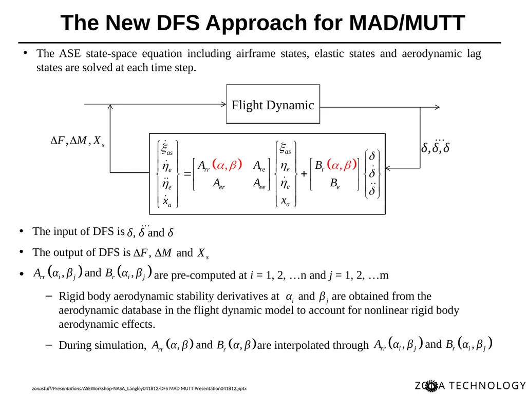
The New DFS Approach for MAD/MUTT The ASE state-space equation including airframe states, elastic states and aerodynamic lag states are solved at each time step. The input of DFS is
The output of DFS is
are pre-computed at i = 1, 2, …n and j = 1, 2, …m
Rigid body aerodynamic stability derivatives at are obtained from the aerodynamic database in the flight dynamic model to account for nonlinear rigid body aerodynamic effects.
During simulation, are interpolated through<br>
The output of DFS is
are pre-computed at i = 1, 2, …n and j = 1, 2, …m
Rigid body aerodynamic stability derivatives at are obtained from the aerodynamic database in the flight dynamic model to account for nonlinear rigid body aerodynamic effects.
During simulation, are interpolated through<br>
20
The and recovery in the original DFS approach does not work for MAD/MUTT.
If [D] matrix in RFA is partitioned into [Drr , Der], the effect of Drr is ignored.
Without Drr, the BFF mode can not be predicted. Instead of computing and from RFA, they can be computed from the structural matrices.
pre-multiplying by yields 0 0 0<br>
If [D] matrix in RFA is partitioned into [Drr , Der], the effect of Drr is ignored.
Without Drr, the BFF mode can not be predicted. Instead of computing and from RFA, they can be computed from the structural matrices.
pre-multiplying by yields 0 0 0<br>
21
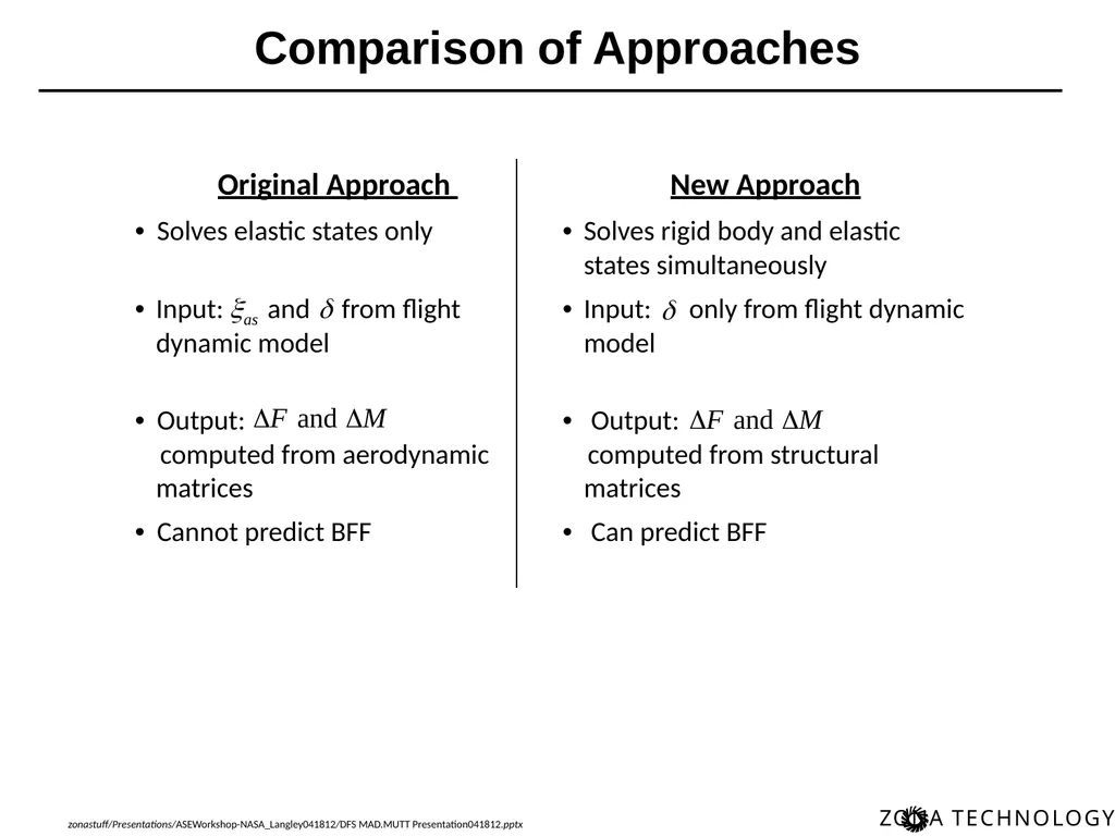
Comparison of Approaches<br>
22
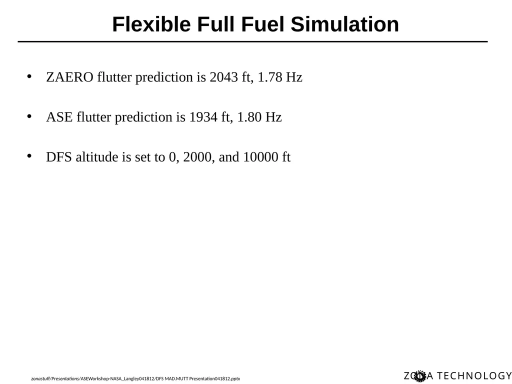
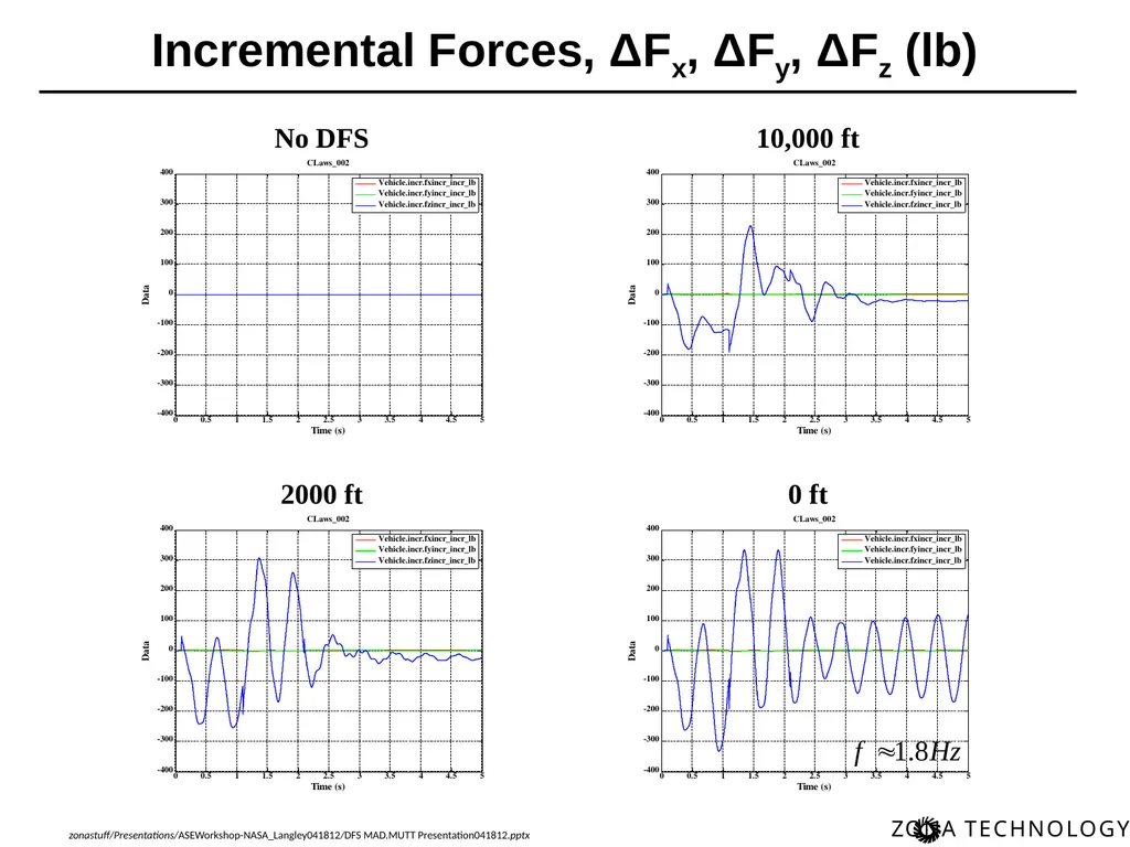
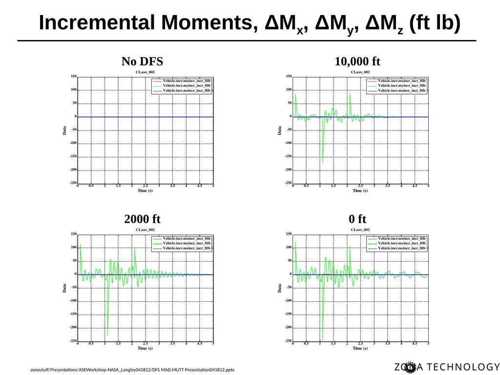
Flexible Full Fuel Simulation ZAERO flutter prediction is 2043 ft, 1.78 Hz
ASE flutter prediction is 1934 ft, 1.80 Hz
DFS altitude is set to 0, 2000, and 10000 ft<br>
ASE flutter prediction is 1934 ft, 1.80 Hz
DFS altitude is set to 0, 2000, and 10000 ft<br>
23
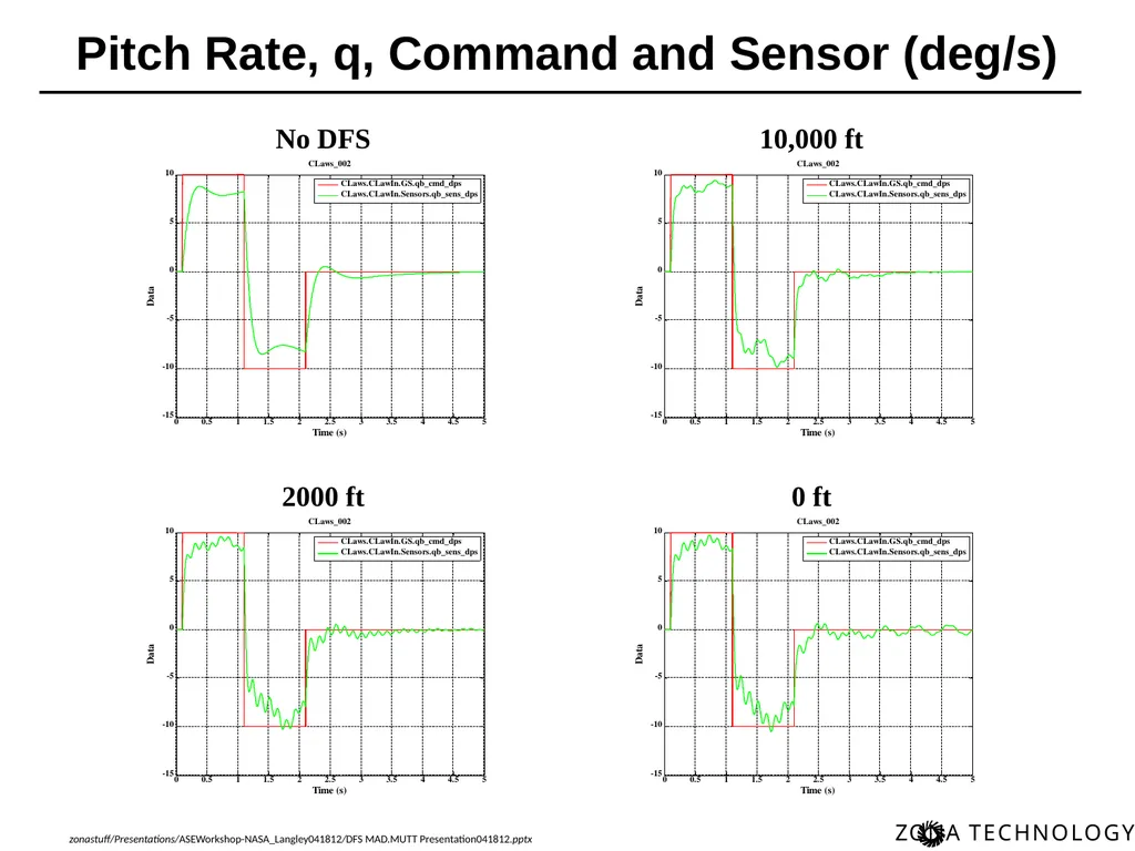
2000 ft 0 ft 10,000 ft No DFS Pitch Rate, q, Command and Sensor (deg/s)<br>
24
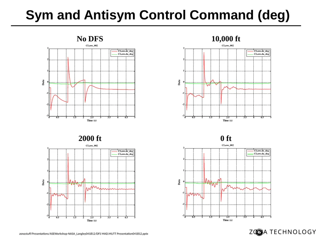
2000 ft 0 ft 10,000 ft No DFS Sym and Antisym Control Command (deg)<br>
25
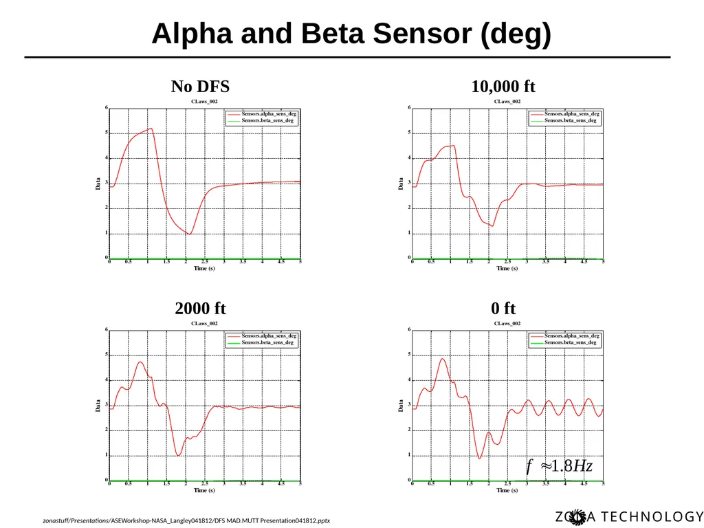
2000 ft 0 ft 10,000 ft No DFS Alpha and Beta Sensor (deg)<br>
26
2000 ft 0 ft 10,000 ft No DFS Incremental Forces, ΔFx, ΔFy, ΔFz (lb)<br>
27
2000 ft 0 ft 10,000 ft No DFS Incremental Moments, ΔMx, ΔMy, ΔMz (ft lb)<br>
28
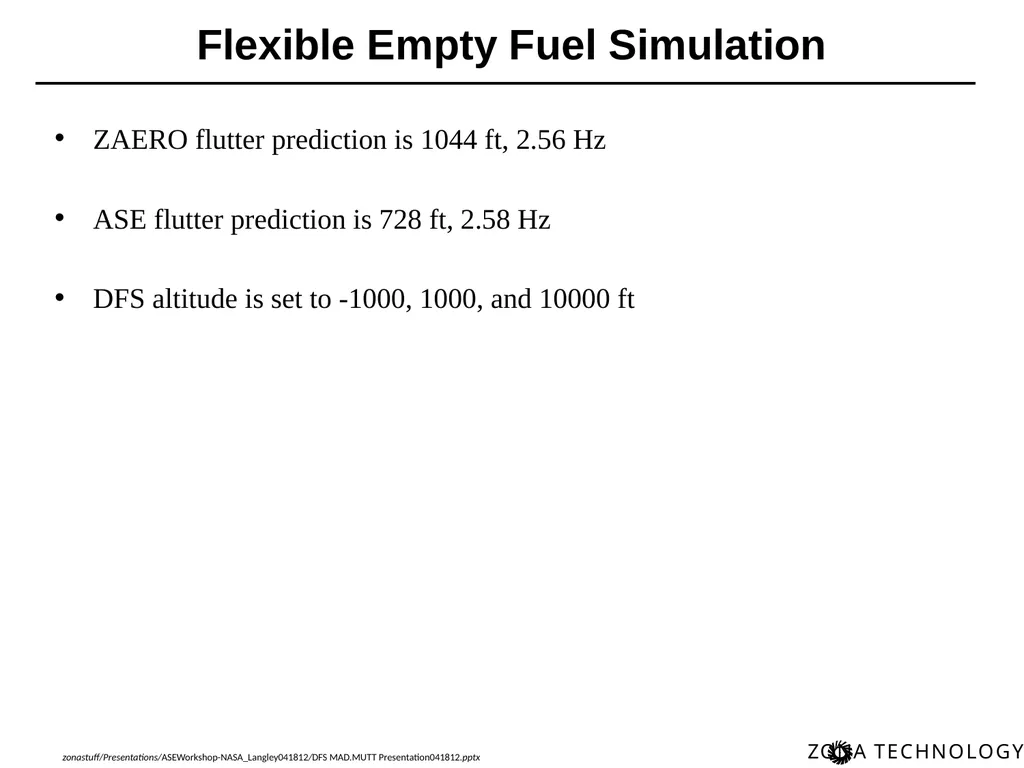
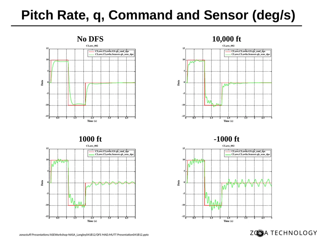
Flexible Empty Fuel Simulation ZAERO flutter prediction is 1044 ft, 2.56 Hz
ASE flutter prediction is 728 ft, 2.58 Hz
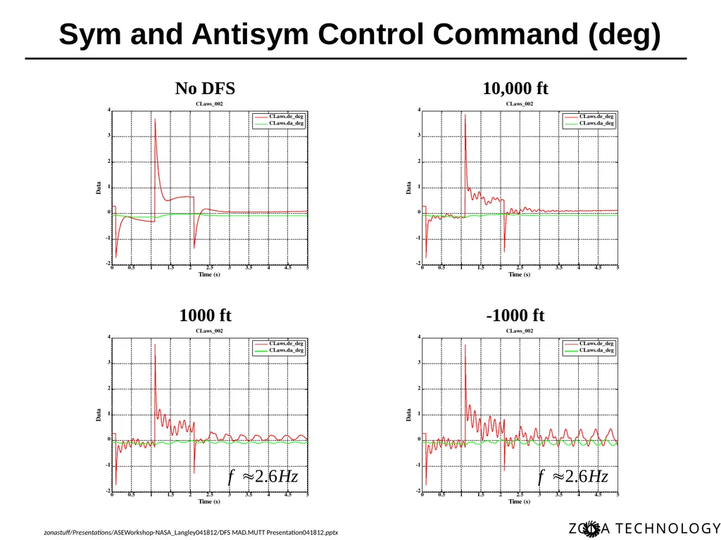
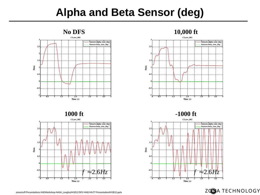
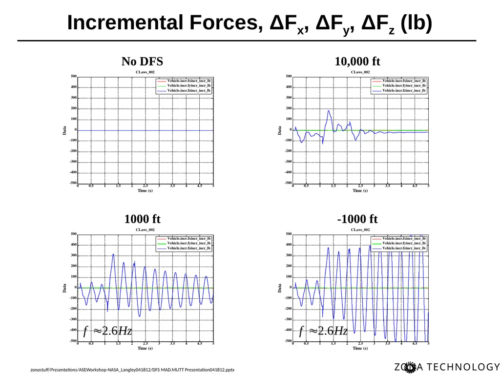
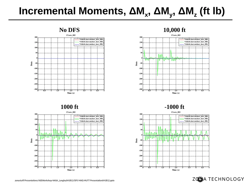
DFS altitude is set to -1000, 1000, and 10000 ft<br>
ASE flutter prediction is 728 ft, 2.58 Hz
DFS altitude is set to -1000, 1000, and 10000 ft<br>
29
1000 ft -1000 ft 10,000 ft No DFS Pitch Rate, q, Command and Sensor (deg/s)<br>
30
1000 ft -1000 ft 10,000 ft No DFS Sym and Antisym Control Command (deg)<br>
31
1000 ft -1000 ft 10,000 ft No DFS Alpha and Beta Sensor (deg)<br>
32
1000 ft -1000 ft 10,000 ft No DFS Incremental Forces, ΔFx, ΔFy, ΔFz (lb)<br>
33
1000 ft -1000 ft 10,000 ft No DFS Incremental Moments, ΔMx, ΔMy, ΔMz (ft lb)<br>
34
Future Work DFS can be used to evaluate the performance of flutter suppression and gust loads alleviation controllers for MAD/MUTT.
So far, the state-space equation in DFS is constructed by the natural modes of each fuel condition.
DFS is defined in different modal coordinates at different fuel conditions.
This allows DFS to perform simulation only one point in the sky at one time.
If the state-space equations at all fuel conditions are constructed by one set of natural modes, for instance of the full fuel condition, DFS can perform a continuous simulation at all flight conditions by a multi-dimensional interpolation.
Through Mach number and altitudes
Through angles of attack and side slip angles
Through fuel conditions
Because of the real-time computational capability of DFS, DFS can be plugged into a real-time simulator to train the pilot under aeroelastic effects.<br>
So far, the state-space equation in DFS is constructed by the natural modes of each fuel condition.
DFS is defined in different modal coordinates at different fuel conditions.
This allows DFS to perform simulation only one point in the sky at one time.
If the state-space equations at all fuel conditions are constructed by one set of natural modes, for instance of the full fuel condition, DFS can perform a continuous simulation at all flight conditions by a multi-dimensional interpolation.
Through Mach number and altitudes
Through angles of attack and side slip angles
Through fuel conditions
Because of the real-time computational capability of DFS, DFS can be plugged into a real-time simulator to train the pilot under aeroelastic effects.<br>