Evaluating a polynomial at a point and Horner’s

mitsue-stanley

Published 2026-09-28 · 21 slides · 0 views

↓ Download

Evaluating a polynomial at a point and Horner’s

Evaluating a polynomial at a point and Horner’s - slide 1 of 21

Evaluating a polynomial at a point and Horner’s - slide 2 of 21

Evaluating a polynomial at a point and Horner’s - slide 3 of 21

Evaluating a polynomial at a point and Horner’s - slide 4 of 21

Evaluating a polynomial at a point and Horner’s - slide 5 of 21

Evaluating a polynomial at a point and Horner’s - slide 6 of 21

Evaluating a polynomial at a point and Horner’s - slide 7 of 21

Evaluating a polynomial at a point and Horner’s - slide 8 of 21

Evaluating a polynomial at a point and Horner’s - slide 9 of 21

Evaluating a polynomial at a point and Horner’s - slide 10 of 21

Evaluating a polynomial at a point and Horner’s - slide 11 of 21

Evaluating a polynomial at a point and Horner’s - slide 12 of 21

Evaluating a polynomial at a point and Horner’s - slide 13 of 21

Evaluating a polynomial at a point and Horner’s - slide 14 of 21

Evaluating a polynomial at a point and Horner’s - slide 15 of 21

Evaluating a polynomial at a point and Horner’s - slide 16 of 21

Evaluating a polynomial at a point and Horner’s - slide 17 of 21

Evaluating a polynomial at a point and Horner’s - slide 18 of 21

Evaluating a polynomial at a point and Horner’s - slide 19 of 21

Evaluating a polynomial at a point and Horner’s - slide 20 of 21

Evaluating a polynomial at a point and Horner’s - slide 21 of 21

Description

Evaluating a polynomial at a point and Horners rule Introduction In this topic, we will Describe the representation of polynomials Discuss the idea of evaluating polynomials Look at a sequence of more efficient implementations We will use

Download this presentation From Below

"Evaluating a polynomial at a point and Horner’s" is the property of its rightful owner. Permission is granted to download and print the materials on this website for personal, non-commercial use only, and to display it on your personal computer provided you do not modify the materials and that you retain all copyright notices contained in the materials. By downloading content from our website, you accept the terms of this agreement.

Presentation Transcript

Evaluating a polynomial at a pointand Horner’s rule

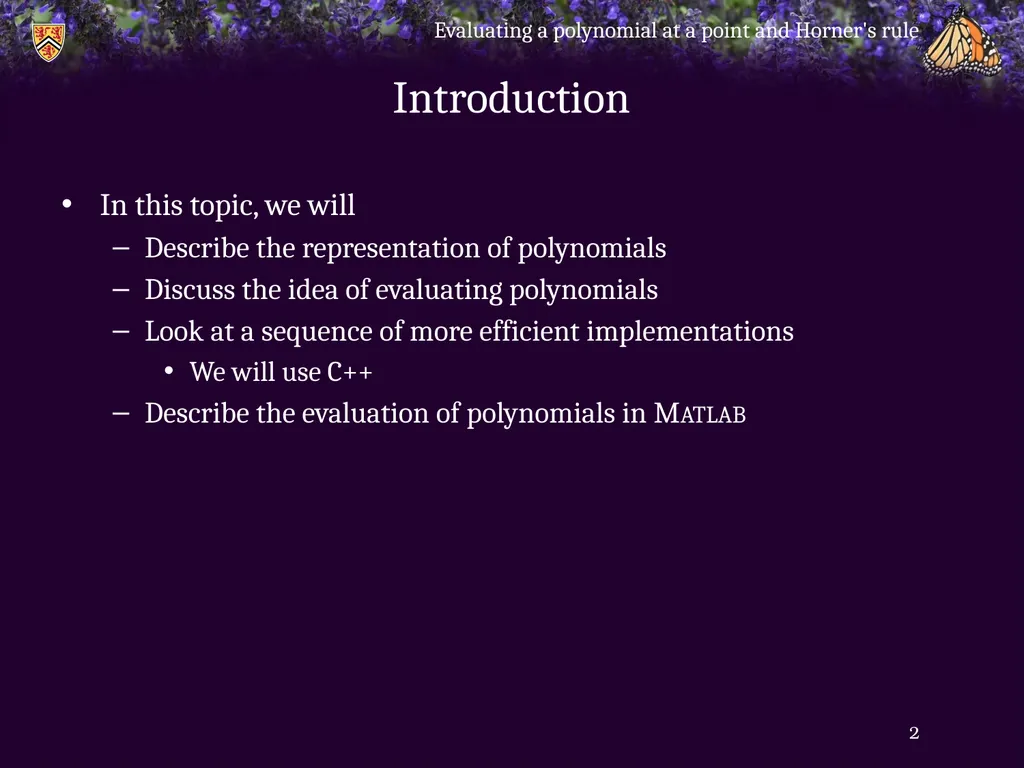
Introduction In this topic, we will
Describe the representation of polynomials
Discuss the idea of evaluating polynomials
Look at a sequence of more efficient implementations
We will use C++
Describe the evaluation of polynomials in Matlab Evaluating a polynomial at a point and Horner's rule 2

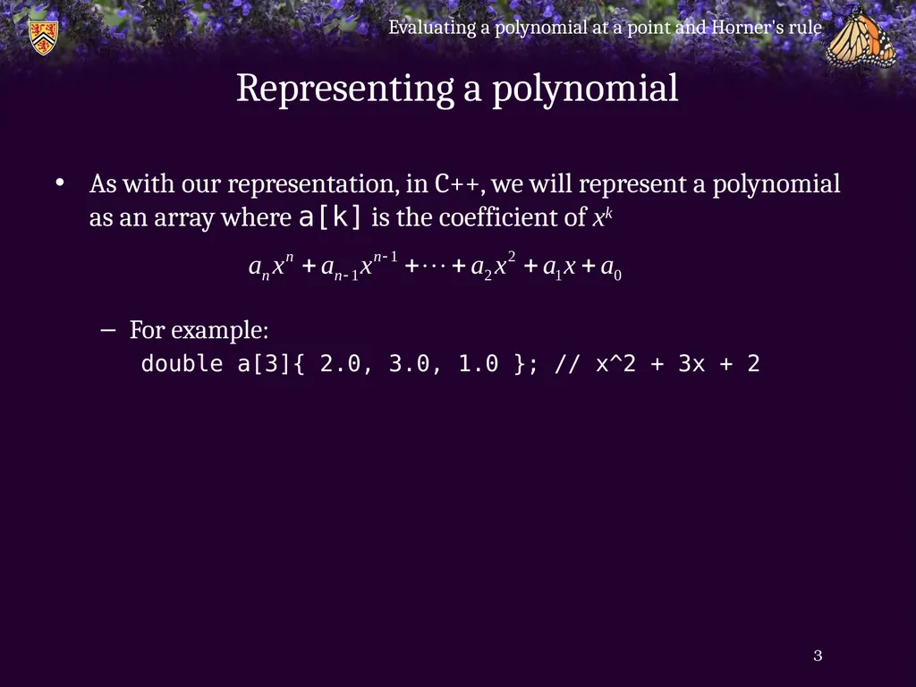
Representing a polynomial As with our representation, in C++, we will represent a polynomial as an array where a[k] is the coefficient of xk

For example:
double a[3]{ 2.0, 3.0, 1.0 }; // x^2 + 3x + 2 Evaluating a polynomial at a point and Horner's rule 3

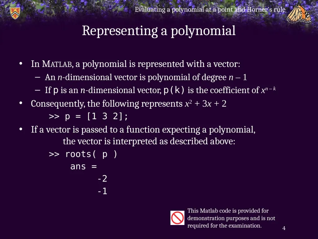
Representing a polynomial In Matlab, a polynomial is represented with a vector:
An n-dimensional vector is polynomial of degree n – 1
If p is an n-dimensional vector, p(k) is the coefficient of xn – k
Consequently, the following represents x2 + 3x + 2
>> p = [1 3 2];
If a vector is passed to a function expecting a polynomial, the vector is interpreted as described above:
>> roots( p )
ans =
-2
-1 Evaluating a polynomial at a point and Horner's rule 4 This Matlab code is provided for demonstration purposes and is not
required for the examination.

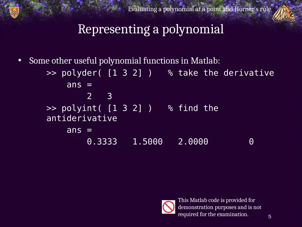
Representing a polynomial Some other useful polynomial functions in Matlab:
>> polyder( [1 3 2] ) % take the derivative
ans =
2 3
>> polyint( [1 3 2] ) % find the antiderivative
ans =
0.3333 1.5000 2.0000 0 Evaluating a polynomial at a point and Horner's rule 5 This Matlab code is provided for demonstration purposes and is not
required for the examination.

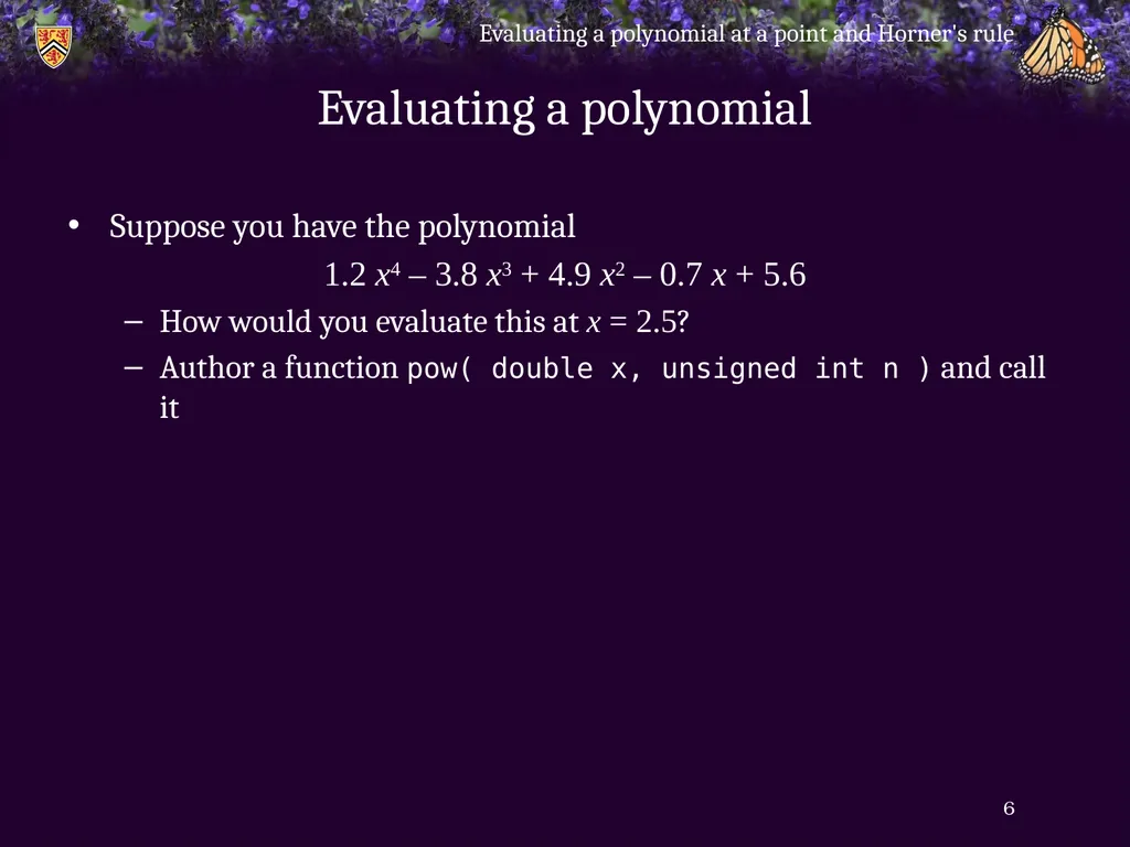
Evaluating a polynomial Suppose you have the polynomial
1.2 x4 – 3.8 x3 + 4.9 x2 – 0.7 x + 5.6
How would you evaluate this at x = 2.5?
Author a function pow( double x, unsigned int n ) and call it Evaluating a polynomial at a point and Horner's rule 6

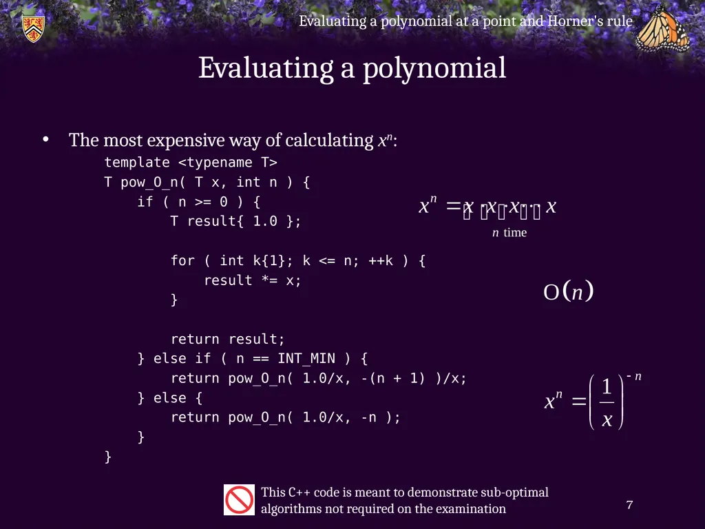
Evaluating a polynomial The most expensive way of calculating xn:
template <typename T>
T pow_O_n( T x, int n ) {
if ( n >= 0 ) {
T result{ 1.0 };

for ( int k{1}; k <= n; ++k ) {
result *= x;
}

return result;
} else if ( n == INT_MIN ) {
return pow_O_n( 1.0/x, -(n + 1) )/x;
} else {
return pow_O_n( 1.0/x, -n );
}
} Evaluating a polynomial at a point and Horner's rule 7 This C++ code is meant to demonstrate sub-optimal algorithms not required on the examination

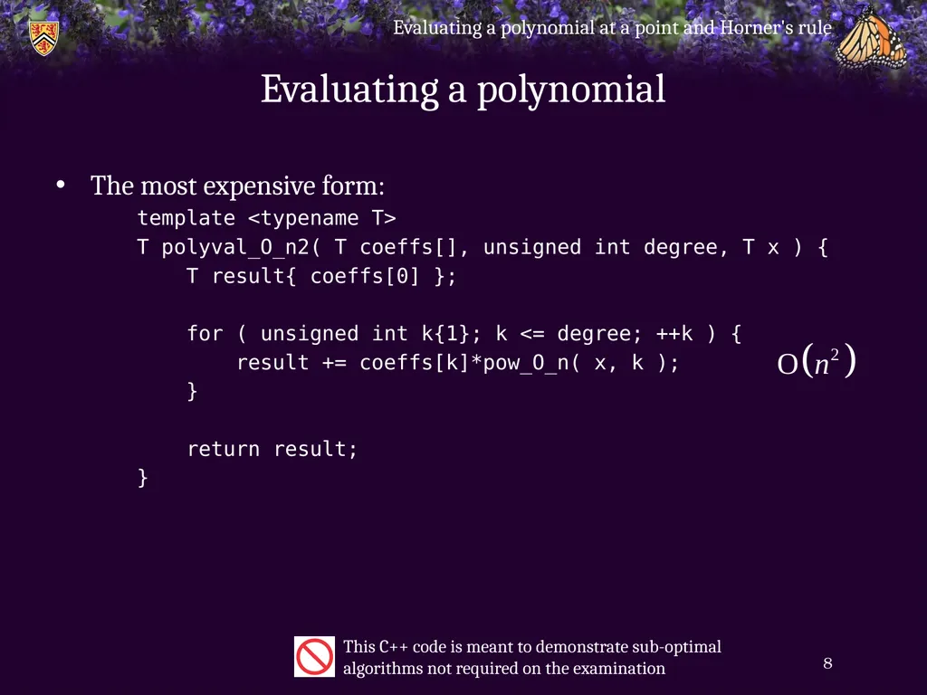
Evaluating a polynomial The most expensive form:
template <typename T>
T polyval_O_n2( T coeffs[], unsigned int degree, T x ) {
T result{ coeffs[0] };

for ( unsigned int k{1}; k <= degree; ++k ) {
result += coeffs[k]*pow_O_n( x, k );
}

return result;
} Evaluating a polynomial at a point and Horner's rule 8 This C++ code is meant to demonstrate sub-optimal algorithms not required on the examination

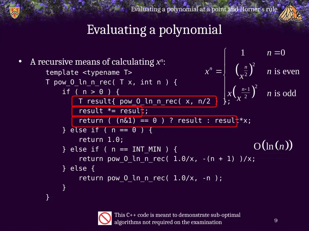
Evaluating a polynomial A recursive means of calculating xn:
template <typename T>
T pow_O_ln_n_rec( T x, int n ) {
if ( n > 0 ) {
T result{ pow_O_ln_n_rec( x, n/2 ) };
result *= result;
return ( (n&1) == 0 ) ? result : result*x;
} else if ( n == 0 ) {
return 1.0;
} else if ( n == INT_MIN ) {
return pow_O_ln_n_rec( 1.0/x, -(n + 1) )/x;
} else {
return pow_O_ln_n_rec( 1.0/x, -n );
}
} Evaluating a polynomial at a point and Horner's rule 9 This C++ code is meant to demonstrate sub-optimal algorithms not required on the examination

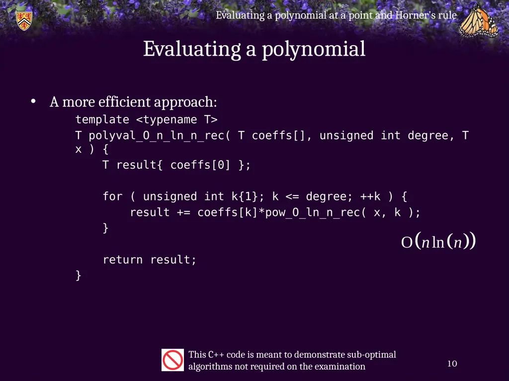
Evaluating a polynomial A more efficient approach:
template <typename T>
T polyval_O_n_ln_n_rec( T coeffs[], unsigned int degree, T x ) {
T result{ coeffs[0] };

for ( unsigned int k{1}; k <= degree; ++k ) {
result += coeffs[k]*pow_O_ln_n_rec( x, k );
}

return result;
} Evaluating a polynomial at a point and Horner's rule 10 This C++ code is meant to demonstrate sub-optimal algorithms not required on the examination

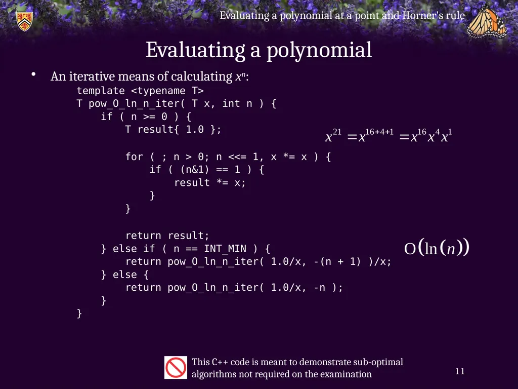
Evaluating a polynomial An iterative means of calculating xn:
template <typename T>
T pow_O_ln_n_iter( T x, int n ) {
if ( n >= 0 ) {
T result{ 1.0 };

for ( ; n > 0; n <<= 1, x *= x ) {
if ( (n&1) == 1 ) {
result *= x;
}
}

return result;
} else if ( n == INT_MIN ) {
return pow_O_ln_n_iter( 1.0/x, -(n + 1) )/x;
} else {
return pow_O_ln_n_iter( 1.0/x, -n );
}
} Evaluating a polynomial at a point and Horner's rule 11 This C++ code is meant to demonstrate sub-optimal algorithms not required on the examination

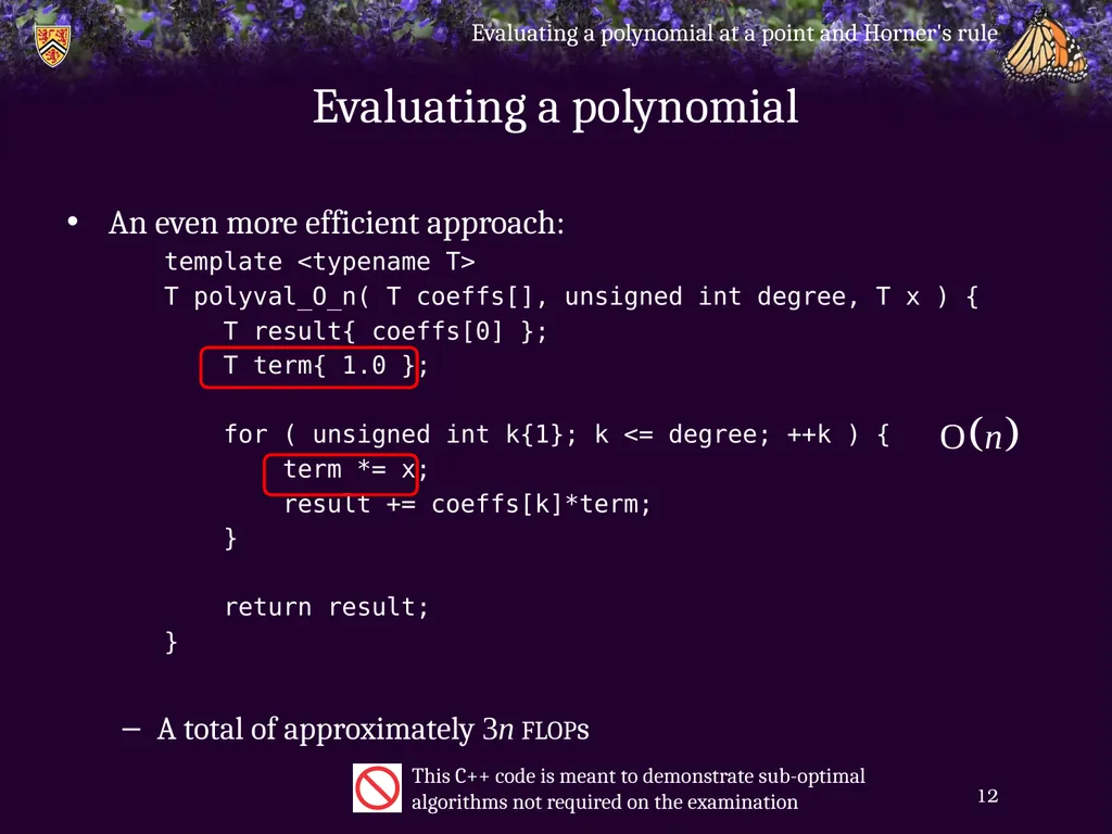
Evaluating a polynomial An even more efficient approach:
template <typename T>
T polyval_O_n( T coeffs[], unsigned int degree, T x ) {
T result{ coeffs[0] };
T term{ 1.0 };

for ( unsigned int k{1}; k <= degree; ++k ) {
term *= x;
result += coeffs[k]*term;
}

return result;
}

A total of approximately 3n flops Evaluating a polynomial at a point and Horner's rule 12 This C++ code is meant to demonstrate sub-optimal algorithms not required on the examination

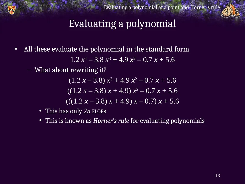
Evaluating a polynomial All these evaluate the polynomial in the standard form
1.2 x4 – 3.8 x3 + 4.9 x2 – 0.7 x + 5.6
What about rewriting it?
(1.2 x – 3.8) x3 + 4.9 x2 – 0.7 x + 5.6
((1.2 x – 3.8) x + 4.9) x2 – 0.7 x + 5.6
(((1.2 x – 3.8) x + 4.9) x – 0.7) x + 5.6
This has only 2n flops
This is known as Horner’s rule for evaluating polynomials Evaluating a polynomial at a point and Horner's rule 13

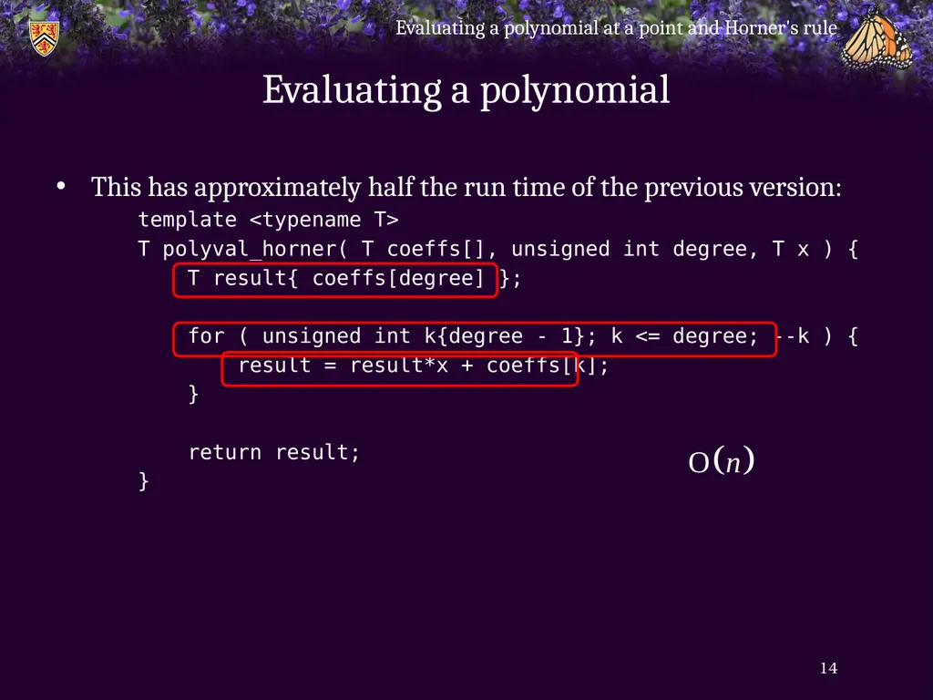
Evaluating a polynomial This has approximately half the run time of the previous version:
template <typename T>
T polyval_horner( T coeffs[], unsigned int degree, T x ) {
T result{ coeffs[degree] };

for ( unsigned int k{degree - 1}; k <= degree; --k ) {
result = result*x + coeffs[k];
}

return result;
} Evaluating a polynomial at a point and Horner's rule 14

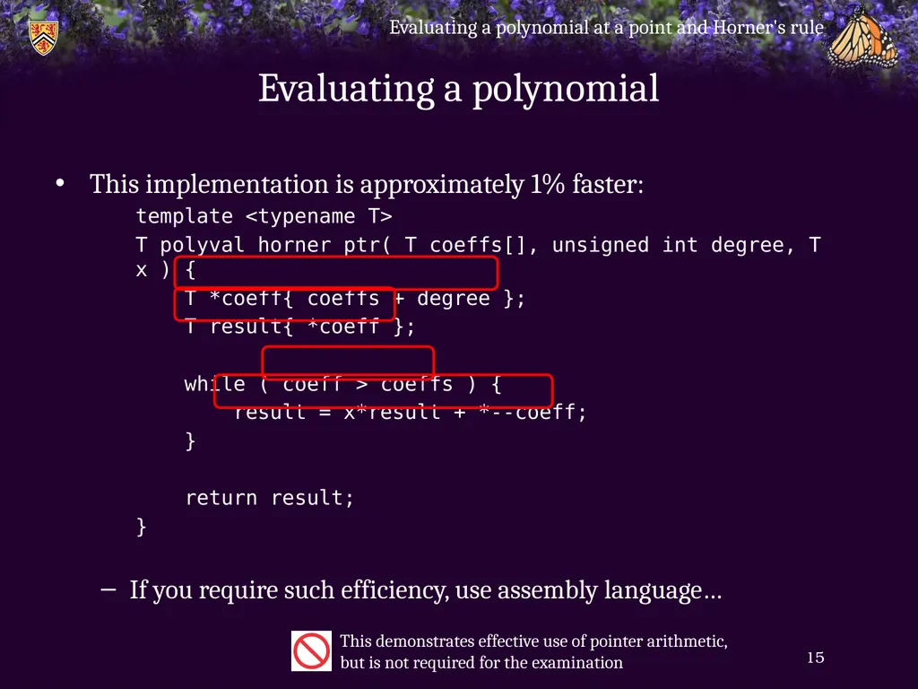
Evaluating a polynomial This implementation is approximately 1% faster:
template <typename T>
T polyval_horner_ptr( T coeffs[], unsigned int degree, T x ) {
T *coeff{ coeffs + degree };
T result{ *coeff };

while ( coeff > coeffs ) {
result = x*result + *--coeff;
}

return result;
}

If you require such efficiency, use assembly language… Evaluating a polynomial at a point and Horner's rule 15 This demonstrates effective use of pointer arithmetic,but is not required for the examination

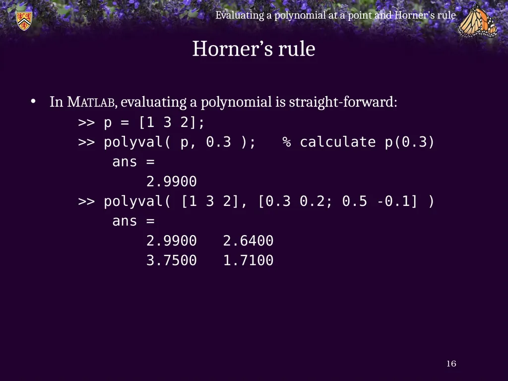
Horner’s rule In Matlab, evaluating a polynomial is straight-forward:
>> p = [1 3 2];
>> polyval( p, 0.3 ); % calculate p(0.3)
ans =
2.9900
>> polyval( [1 3 2], [0.3 0.2; 0.5 -0.1] )
ans =
2.9900 2.6400
3.7500 1.7100 Evaluating a polynomial at a point and Horner's rule 16

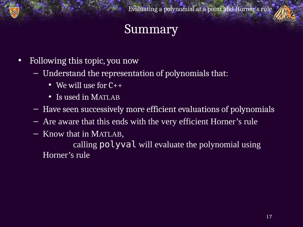
Summary Following this topic, you now
Understand the representation of polynomials that:
We will use for C++
Is used in Matlab
Have seen successively more efficient evaluations of polynomials
Are aware that this ends with the very efficient Horner’s rule
Know that in Matlab, calling polyval will evaluate the polynomial using Horner’s rule Evaluating a polynomial at a point and Horner's rule 17

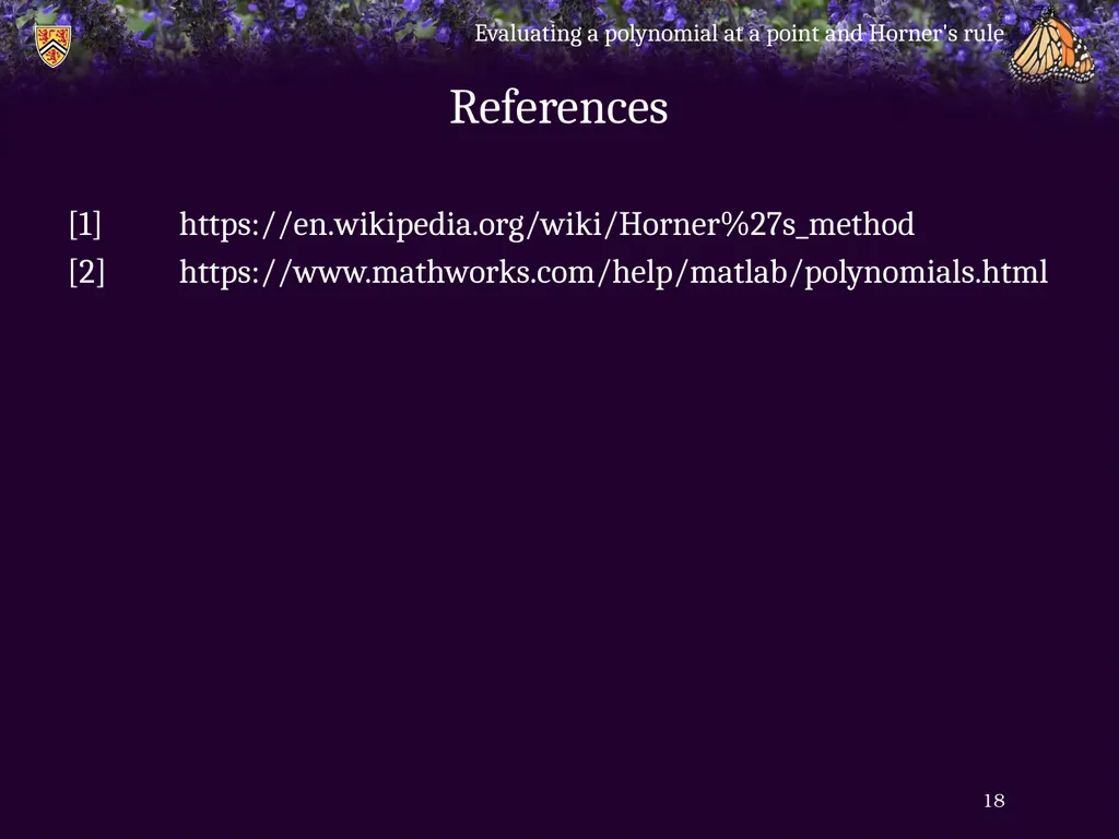
References [1] https://en.wikipedia.org/wiki/Horner%27s_method
[2] https://www.mathworks.com/help/matlab/polynomials.html Evaluating a polynomial at a point and Horner's rule 18

Acknowledgments None so far. Evaluating a polynomial at a point and Horner's rule 19

Colophon These slides were prepared using the Cambria typeface. Mathematical equations use Times New Roman, and source code is presented using Consolas. Mathematical equations are prepared in MathType by Design Science, Inc.
Examples may be formulated and checked using Maple by Maplesoft, Inc.

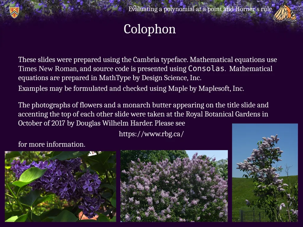
The photographs of flowers and a monarch butter appearing on the title slide and accenting the top of each other slide were taken at the Royal Botanical Gardens in October of 2017 by Douglas Wilhelm Harder. Please see
https://www.rbg.ca/
for more information. Evaluating a polynomial at a point and Horner's rule 20

Disclaimer These slides are provided for the ece 204 Numerical methods course taught at the University of Waterloo. The material in it reflects the author’s best judgment in light of the information available to them at the time of preparation. Any reliance on these course slides by any party for any other purpose are the responsibility of such parties. The authors accept no responsibility for damages, if any, suffered by any party as a result of decisions made or actions based on these course slides for any other purpose than that for which it was intended. Evaluating a polynomial at a point and Horner's rule 21

Evaluating a polynomial at a point and Horner’s

Related Topics

Share

Embed code

Download this presentation From Below

Presentation Transcript