Expectation Maximization CS771: Introduction to
Description: Expectation Maximization CS771: Introduction to Machine Learning Nisheeth Building intuition for EM: a case study Let events be grades in a class w1 Gets an A P(A) ½ w2 Gets a B P(B) μ w3 Gets a C P(C) 2μ w4 Gets a D P(D)
Related Topics
Download Presentation
"Expectation Maximization CS771: Introduction to" is the property of its rightful owner. Permission is granted to download and print the materials on this website for personal, non-commercial use only, and to display it on your personal computer provided you do not modify the materials and that you retain all copyright notices contained in the materials. By downloading content from our website, you accept the terms of this agreement.
Presentation Transcript
slide1. Expectation Maximization CS771: Introduction to Machine Learning
Nisheeth<br>
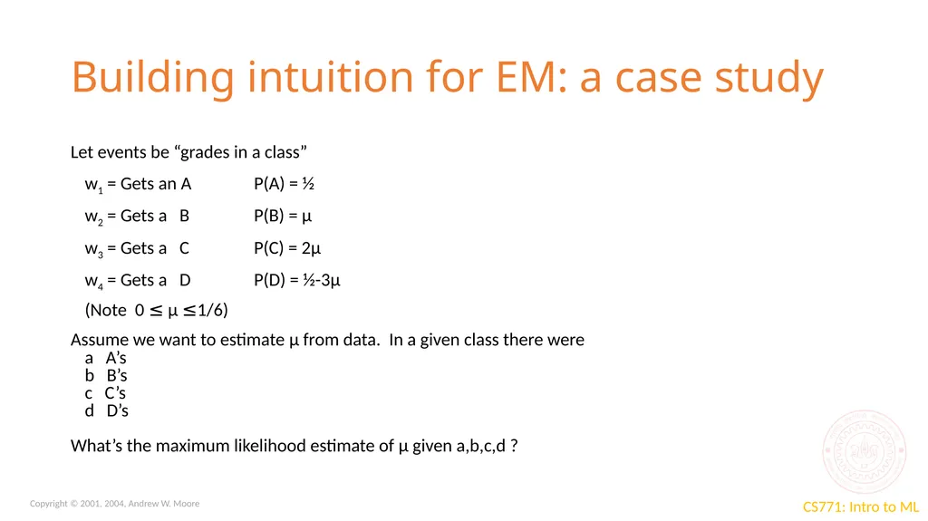
slide2. Building intuition for EM: a case study Let events be “grades in a class”
w1 = Gets an A P(A) = ½
w2 = Gets a B P(B) = μ
w3 = Gets a C P(C) = 2μ
w4 = Gets a D P(D) = ½-3μ
(Note 0 ≤ μ ≤1/6)
Assume we want to estimate μ from data. In a given class there were
a A’s
b B’s
c C’s
d D’s
What’s the maximum likelihood estimate of μ given a,b,c,d ? Copyright © 2001, 2004, Andrew W. Moore<br>
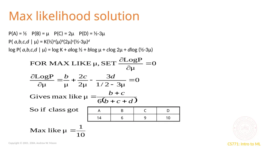
slide3. Max likelihood solution P(A) = ½ P(B) = μ P(C) = 2μ P(D) = ½-3μ
P( a,b,c,d | μ) = K(½)a(μ)b(2μ)c(½-3μ)d
log P( a,b,c,d | μ) = log K + alog ½ + blog μ + clog 2μ + dlog (½-3μ) Copyright © 2001, 2004, Andrew W. Moore<br>
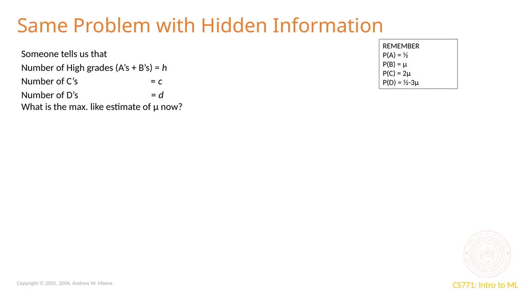
slide4. Same Problem with Hidden Information Someone tells us that
Number of High grades (A’s + B’s) = h
Number of C’s = c
Number of D’s = d
What is the max. like estimate of μ now? REMEMBER
P(A) = ½
P(B) = μ
P(C) = 2μ
P(D) = ½-3μ Copyright © 2001, 2004, Andrew W. Moore<br>
slide5. Same Problem with Hidden Information Someone tells us that
Number of High grades (A’s + B’s) = h
Number of C’s = c
Number of D’s = d
What is the max. like estimate of μ now?
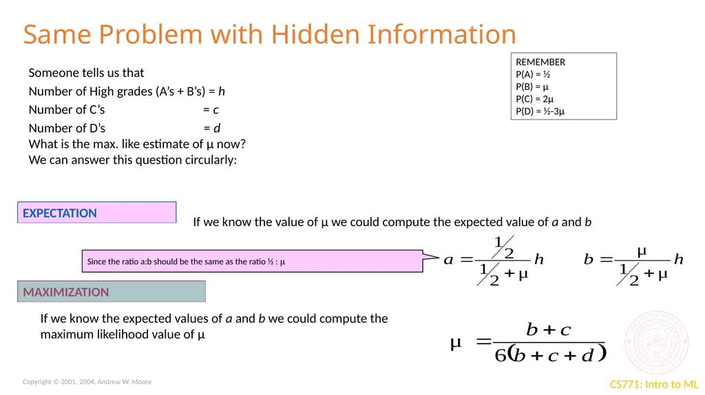
We can answer this question circularly: EXPECTATION MAXIMIZATION If we know the value of μ we could compute the expected value of a and b If we know the expected values of a and b we could compute the maximum likelihood value of μ REMEMBER
P(A) = ½
P(B) = μ
P(C) = 2μ
P(D) = ½-3μ Since the ratio a:b should be the same as the ratio ½ : m Copyright © 2001, 2004, Andrew W. Moore<br>
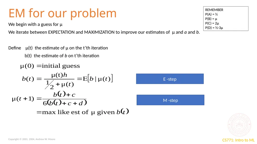
slide6. EM for our problem We begin with a guess for μ
We iterate between EXPECTATION and MAXIMIZATION to improve our estimates of μ and a and b.
Define μ(t) the estimate of μ on the t’th iteration
b(t) the estimate of b on t’th iteration REMEMBER
P(A) = ½
P(B) = μ
P(C) = 2μ
P(D) = ½-3μ Copyright © 2001, 2004, Andrew W. Moore E -step M -step<br>
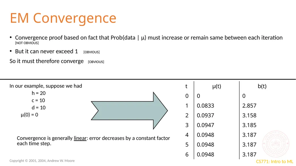
slide7. Copyright © 2001, 2004, Andrew W. Moore EM Convergence Convergence proof based on fact that Prob(data | μ) must increase or remain same between each iteration [NOT OBVIOUS]
But it can never exceed 1 [OBVIOUS]
So it must therefore converge [OBVIOUS] In our example, suppose we had
h = 20
c = 10
d = 10
μ(0) = 0 Convergence is generally linear: error decreases by a constant factor each time step.<br>
slide8. ALT-OPT/EM for Gaussian Mixture Model 8<br>
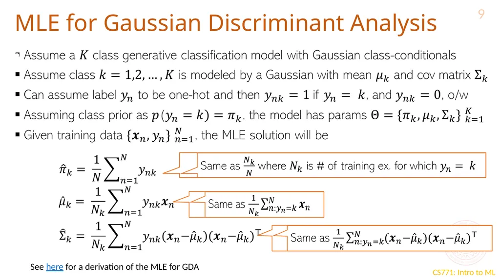
slide9. MLE for Gaussian Discriminant Analysis 9 See here for a derivation of the MLE for GDA<br>
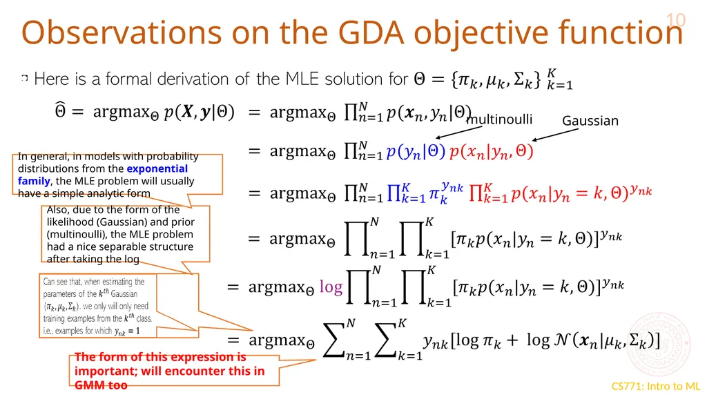
slide10. Observations on the GDA objective function 10 multinoulli Gaussian Also, due to the form of the likelihood (Gaussian) and prior (multinoulli), the MLE problem had a nice separable structure after taking the log In general, in models with probability distributions from the exponential family, the MLE problem will usually have a simple analytic form The form of this expression is important; will encounter this in GMM too<br>
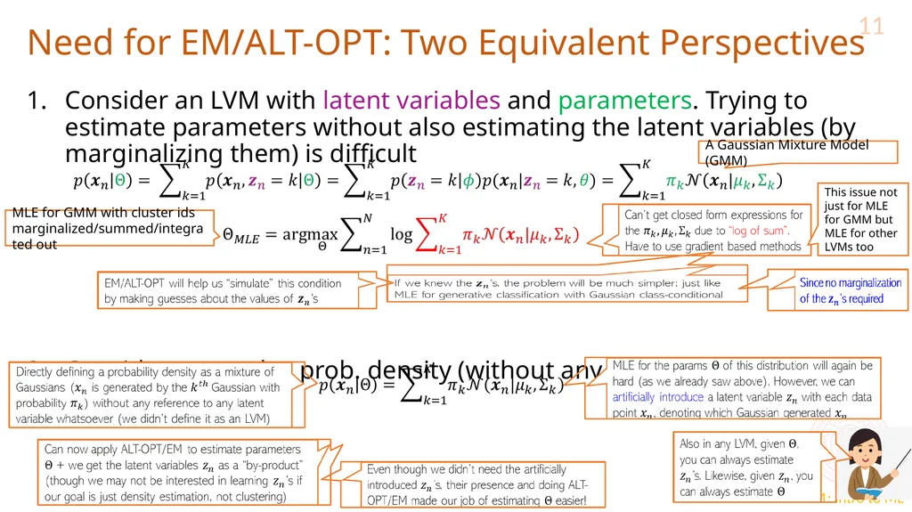
slide11. Need for EM/ALT-OPT: Two Equivalent Perspectives 11 Consider an LVM with latent variables and parameters. Trying to estimate parameters without also estimating the latent variables (by marginalizing them) is difficult
Consider a complex prob. density (without any latent vars) for which MLE is hard A Gaussian Mixture Model (GMM) MLE for GMM with cluster ids marginalized/summed/integrated out This issue not just for MLE for GMM but MLE for other LVMs too<br>
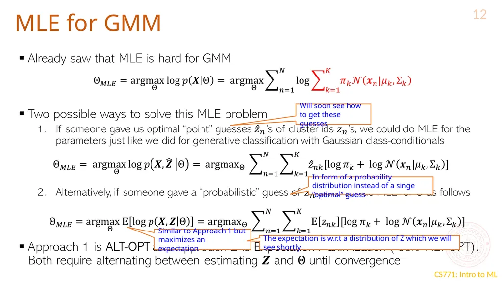
slide12. MLE for GMM 12 Will soon see how to get these guesses Similar to Approach 1 but maximizes an expectation The expectation is w.r.t a distribution of Z which we will see shortly In form of a probability distribution instead of a singe “optimal” guess<br>
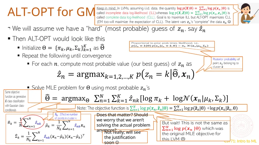
slide13. ALT-OPT for GMM 13 Does that matter? Should we worry that we aren’t solving the actual problem anymore? Not really; will see the justification soon <br>
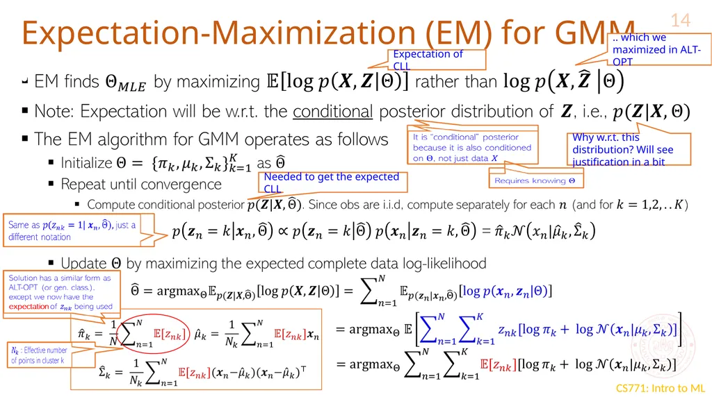
slide14. Expectation-Maximization (EM) for GMM 14 .. which we maximized in ALT-OPT Expectation of CLL Why w.r.t. this distribution? Will see justification in a bit Needed to get the expected CLL<br>
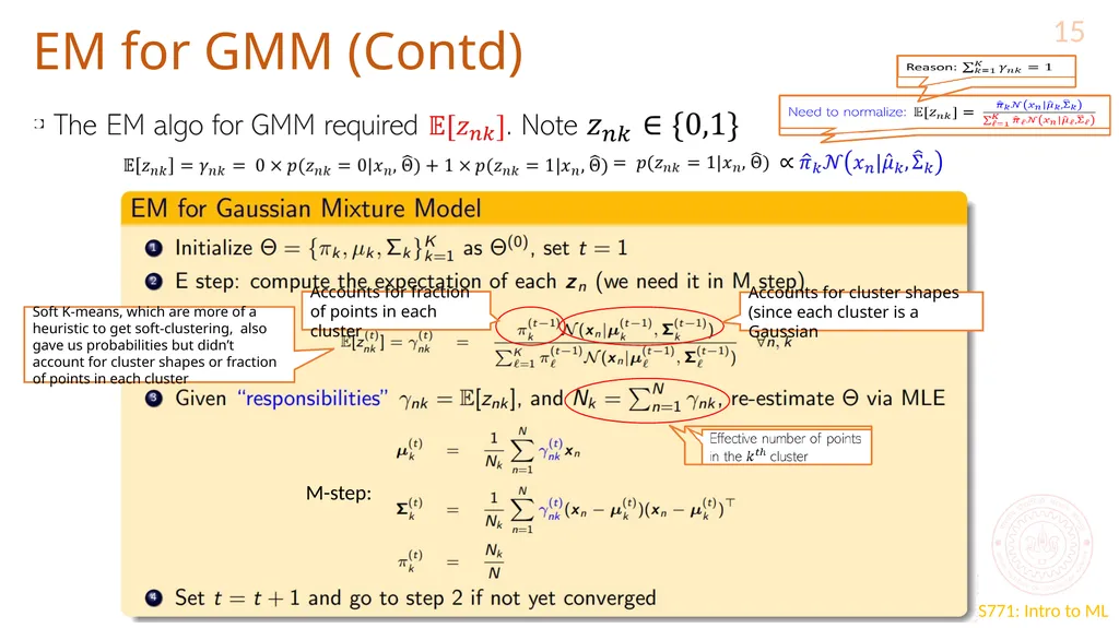
slide15. EM for GMM (Contd) 15 M-step: Soft K-means, which are more of a heuristic to get soft-clustering, also gave us probabilities but didn’t account for cluster shapes or fraction of points in each cluster Accounts for cluster shapes (since each cluster is a Gaussian Accounts for fraction of points in each cluster<br>
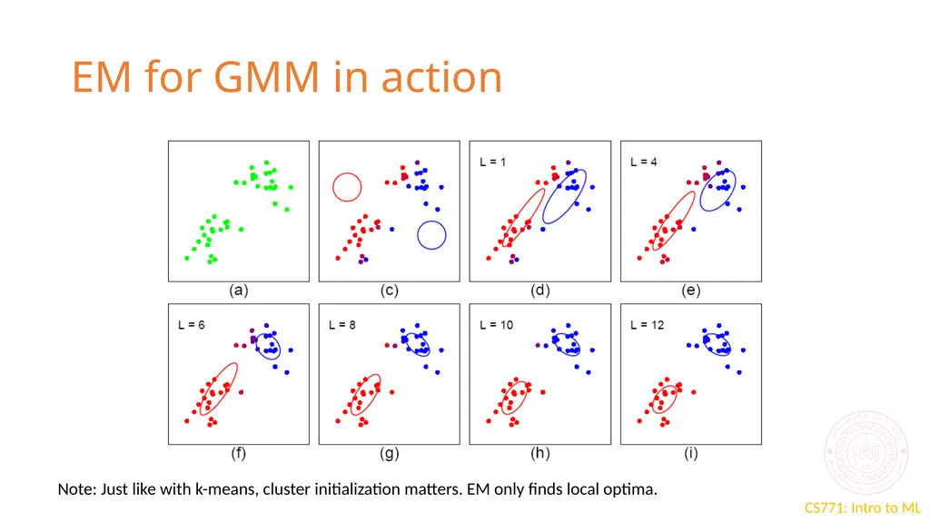
slide16. EM for GMM in action Note: Just like with k-means, cluster initialization matters. EM only finds local optima.<br>

Nisheeth<br>
slide2. Building intuition for EM: a case study Let events be “grades in a class”
w1 = Gets an A P(A) = ½
w2 = Gets a B P(B) = μ
w3 = Gets a C P(C) = 2μ
w4 = Gets a D P(D) = ½-3μ
(Note 0 ≤ μ ≤1/6)
Assume we want to estimate μ from data. In a given class there were
a A’s
b B’s
c C’s
d D’s
What’s the maximum likelihood estimate of μ given a,b,c,d ? Copyright © 2001, 2004, Andrew W. Moore<br>
slide3. Max likelihood solution P(A) = ½ P(B) = μ P(C) = 2μ P(D) = ½-3μ
P( a,b,c,d | μ) = K(½)a(μ)b(2μ)c(½-3μ)d
log P( a,b,c,d | μ) = log K + alog ½ + blog μ + clog 2μ + dlog (½-3μ) Copyright © 2001, 2004, Andrew W. Moore<br>
slide4. Same Problem with Hidden Information Someone tells us that
Number of High grades (A’s + B’s) = h
Number of C’s = c
Number of D’s = d
What is the max. like estimate of μ now? REMEMBER
P(A) = ½
P(B) = μ
P(C) = 2μ
P(D) = ½-3μ Copyright © 2001, 2004, Andrew W. Moore<br>
slide5. Same Problem with Hidden Information Someone tells us that
Number of High grades (A’s + B’s) = h
Number of C’s = c
Number of D’s = d
What is the max. like estimate of μ now?
We can answer this question circularly: EXPECTATION MAXIMIZATION If we know the value of μ we could compute the expected value of a and b If we know the expected values of a and b we could compute the maximum likelihood value of μ REMEMBER
P(A) = ½
P(B) = μ
P(C) = 2μ
P(D) = ½-3μ Since the ratio a:b should be the same as the ratio ½ : m Copyright © 2001, 2004, Andrew W. Moore<br>
slide6. EM for our problem We begin with a guess for μ
We iterate between EXPECTATION and MAXIMIZATION to improve our estimates of μ and a and b.
Define μ(t) the estimate of μ on the t’th iteration
b(t) the estimate of b on t’th iteration REMEMBER
P(A) = ½
P(B) = μ
P(C) = 2μ
P(D) = ½-3μ Copyright © 2001, 2004, Andrew W. Moore E -step M -step<br>
slide7. Copyright © 2001, 2004, Andrew W. Moore EM Convergence Convergence proof based on fact that Prob(data | μ) must increase or remain same between each iteration [NOT OBVIOUS]
But it can never exceed 1 [OBVIOUS]
So it must therefore converge [OBVIOUS] In our example, suppose we had
h = 20
c = 10
d = 10
μ(0) = 0 Convergence is generally linear: error decreases by a constant factor each time step.<br>
slide8. ALT-OPT/EM for Gaussian Mixture Model 8<br>
slide9. MLE for Gaussian Discriminant Analysis 9 See here for a derivation of the MLE for GDA<br>
slide10. Observations on the GDA objective function 10 multinoulli Gaussian Also, due to the form of the likelihood (Gaussian) and prior (multinoulli), the MLE problem had a nice separable structure after taking the log In general, in models with probability distributions from the exponential family, the MLE problem will usually have a simple analytic form The form of this expression is important; will encounter this in GMM too<br>
slide11. Need for EM/ALT-OPT: Two Equivalent Perspectives 11 Consider an LVM with latent variables and parameters. Trying to estimate parameters without also estimating the latent variables (by marginalizing them) is difficult
Consider a complex prob. density (without any latent vars) for which MLE is hard A Gaussian Mixture Model (GMM) MLE for GMM with cluster ids marginalized/summed/integrated out This issue not just for MLE for GMM but MLE for other LVMs too<br>
slide12. MLE for GMM 12 Will soon see how to get these guesses Similar to Approach 1 but maximizes an expectation The expectation is w.r.t a distribution of Z which we will see shortly In form of a probability distribution instead of a singe “optimal” guess<br>
slide13. ALT-OPT for GMM 13 Does that matter? Should we worry that we aren’t solving the actual problem anymore? Not really; will see the justification soon <br>
slide14. Expectation-Maximization (EM) for GMM 14 .. which we maximized in ALT-OPT Expectation of CLL Why w.r.t. this distribution? Will see justification in a bit Needed to get the expected CLL<br>
slide15. EM for GMM (Contd) 15 M-step: Soft K-means, which are more of a heuristic to get soft-clustering, also gave us probabilities but didn’t account for cluster shapes or fraction of points in each cluster Accounts for cluster shapes (since each cluster is a Gaussian Accounts for fraction of points in each cluster<br>
slide16. EM for GMM in action Note: Just like with k-means, cluster initialization matters. EM only finds local optima.<br>