Graphing Interactions Using the PROCESS Macro in

slide1. Graphing Interactions Using the PROCESS Macro in SPSS Christine R. Wells, Ph.D.
UCLA Office of Advanced Research Computing
Statistical Methods and Data Analytics<br>
slide2. Introduction We will cover only some of what can be done in the PROCESS macro in SPSS.
We will focus on moderation models (no mediation).
We will be using version 4.0 of the PROCESS macro.
Information about the PROCESS macro can be found at https://www.processmacro.org/index.html
Much of the material in this workshop is based on Introduction to Mediation, Moderation and Conditional Process Analysis: A Regression-based Approach, Third Edition by Andrew F. Hayes (2022).<br>
slide3. Installing PROCESS Go to processmacro.org and then to the Downloads tab (at the top of the page).
Download the zipped file, and then unzip the file.
Read the Installing PROCESS custom dialog PDF.
Finally, open and run the process.sps file.
The custom dialog will remain installed as you open and close the SPSS program, but you must run the process.sps file each time you open SPSS and want to use the PROCESS macro.<br>
slide4. Download the datasets Please go to the webpage and download the datasets hsbmoderation.sav and exercise.sav.
Save them somewhere that it is easy for you to access (such as C:\).
NOTE: SPSS will allow long variable names, but PROCESS has trouble with variable names longer than eight characters. To avoid these potential difficulties, the names of all variables used in the examples are eight characters or less.<br>
slide5. Getting the SPSS commands in the log file Log file = output file
Some versions of SPSS have the syntax echoed in the output by default.
If you don’t see SPSS syntax above the output, click on Edit, Options, the Viewer tab, and then click to check the box in lower left corner to Display the Commands in the Log.<br>
slide6. Definition of interaction term Interaction terms are common in regression models.
Without an interaction term in a regression model, the effect of one predictor on the outcome is independent of all other predictors in the model.
The interaction term is the product of two predictors.
The inclusion of an interaction term in a regression model means that the effect of one predictor on the outcome depends on the level of the other predictor.<br>
slide7. Definition of interaction term (continued) Interaction terms are symmetric: the effect of Predictor A on the outcome depends on the level of Predictor B, and the effect of Predictor B on the outcome depends on the level of Predictor A.
For simplicity, some authors refer to one predictor as “the predictor” and the other as “the moderator”.
The important thing to remember is that those names are used only to help people; there is no difference mathematically and your statistical software does not care what you call any of the predictors.<br>
slide8. In this workshop You will learn how to interpret the coefficients of the interaction terms and the lower-order effects (to be explained later), how to probe the interaction and how to graph it.
Many researchers find the interpretation of the coefficients of the interaction terms to be difficult, so they simply report whether or not the term is statistically significant and then present the graph of the interaction.<br>
slide9. SPSS procedures to run linear regression There are many procedures that can be used to run linear regression analyses in SPSS, e.g., REGRESSION, GLM, MIXED, LINEAR.
However, most procedures that run regression analyses in SPSS lack the ability to graph interactions.
One exception to this is the GLM command, which can graph binary-by-binary interactions.
This is a big limitation, so we will use PROCESS to graph interactions that SPSS can’t.<br>
slide10. Graphing interactions with PROCESS The PROCESS macro, written by Andrew Hayes, provides a way to get the information necessary to graph a variety of different types of interactions, including binary-by-binary, binary-by-continuous, continuous-by-continuous, two two-way interactions in a model and even three-way interactions.
This workshop will focus on graphing different types of interactions in linear regression models.<br>
slide11. The datasets Hsbmoderation
outcome = opinion
predictors = detail, age, etc.
Exercise
outcome = loss
predictors = hours, effort, female<br>
slide12. DATASET NAME and DATASET ACTIVATE Before we start using the PROCESS macro, we need to quickly discuss some SPSS commands that we will need to keep everything running correctly.
The SPSS command DATASET NAME is used to name a dataset that has been created (but not necessarily saved anywhere).
The SPSS command DATASET ACTIVATE makes active a particular dataset, and this will be used to ensure that the correct dataset is active just before we execute the SPSS syntax.<br>
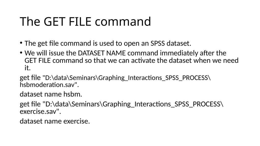
slide13. The GET FILE command The get file command is used to open an SPSS dataset.
We will issue the DATASET NAME command immediately after the GET FILE command so that we can activate the dataset when we need it.
get file "D:\data\Seminars\Graphing_Interactions_SPSS_PROCESS\hsbmoderation.sav".
dataset name hsbm.
get file "D:\data\Seminars\Graphing_Interactions_SPSS_PROCESS\exercise.sav".
dataset name exercise.<br>
slide14. Binary by binary interactions<br>
slide15. Interaction and lower-order terms The interaction term is the product of two predictors, binaryvr and bcovar.
The variables binaryvr and bcovar will also be included in the model; they are called “lower-order” terms.
Their presence in the model is necessary to make the coefficient of the interaction term interpretable.
Hence there are three predictor variables: binaryvr, bcovar and their interaction.
Do not use recoded versions of the lower-order effects.<br>
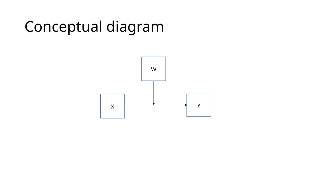
slide16. Conceptual diagram W X Y<br>
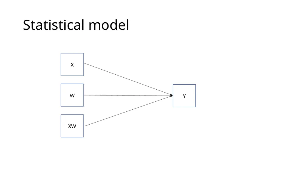
slide17. Statistical model X W XW Y<br>
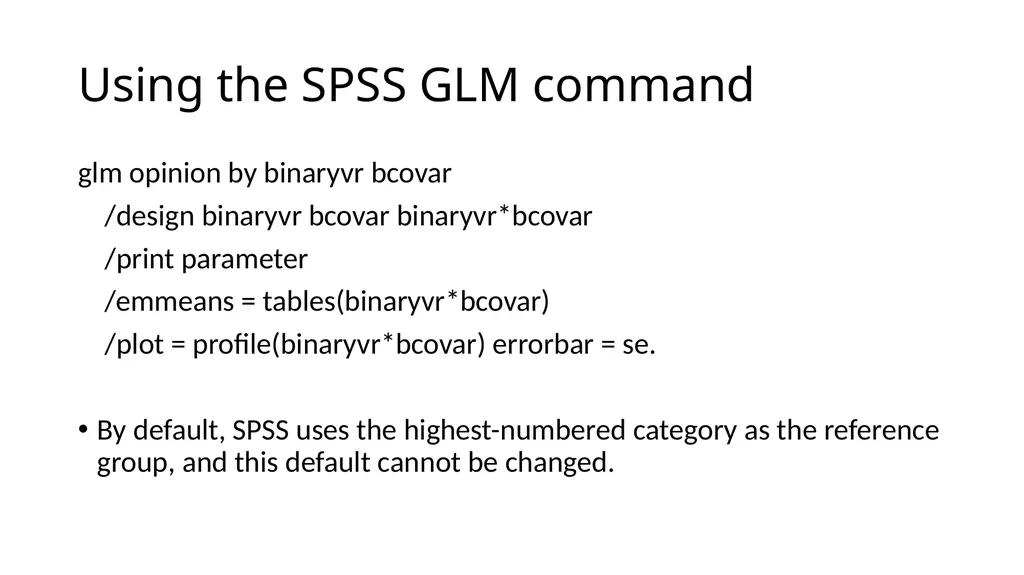
slide18. Using the SPSS GLM command glm opinion by binaryvr bcovar
/design binaryvr bcovar binaryvr*bcovar
/print parameter
/emmeans = tables(binaryvr*bcovar)
/plot = profile(binaryvr*bcovar) errorbar = se.

By default, SPSS uses the highest-numbered category as the reference group, and this default cannot be changed.<br>
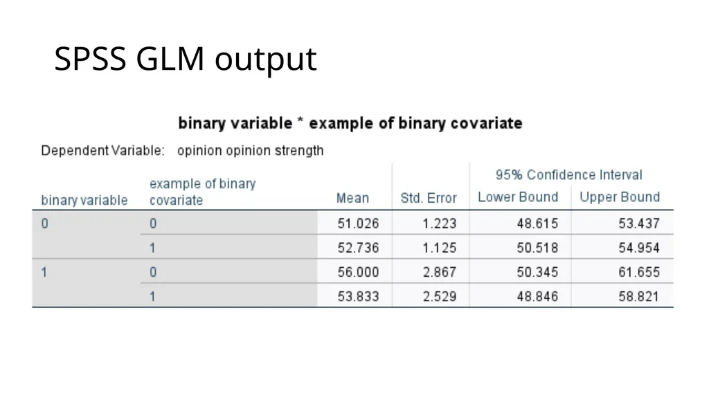
slide19. SPSS GLM output<br>
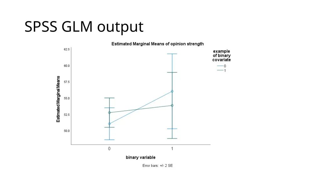
slide20. SPSS GLM output<br>
slide21. SPSS GLM output<br>
slide22. SPSS GLM output<br>
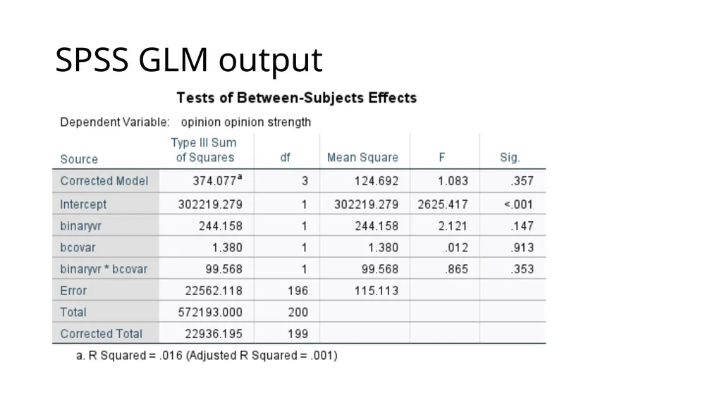
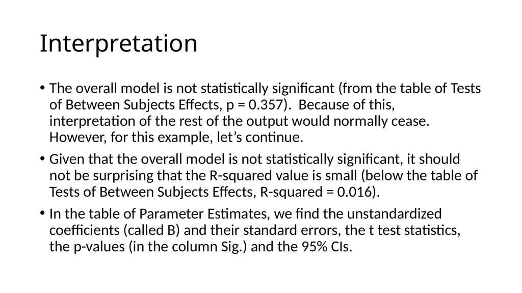
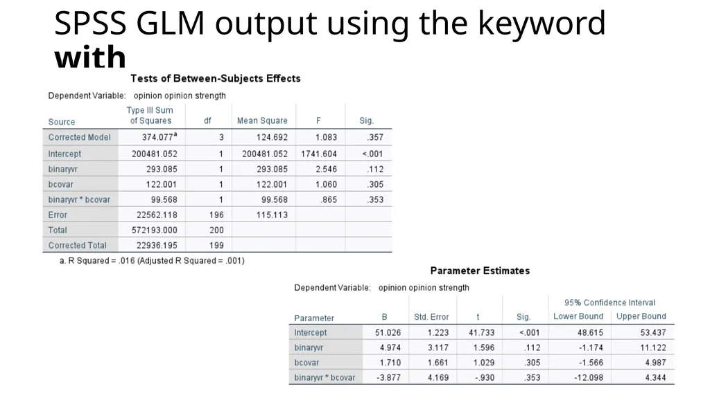
slide23. Interpretation The overall model is not statistically significant (from the table of Tests of Between Subjects Effects, p = 0.357). Because of this, interpretation of the rest of the output would normally cease. However, for this example, let’s continue.
Given that the overall model is not statistically significant, it should not be surprising that the R-squared value is small (below the table of Tests of Between Subjects Effects, R-squared = 0.016).
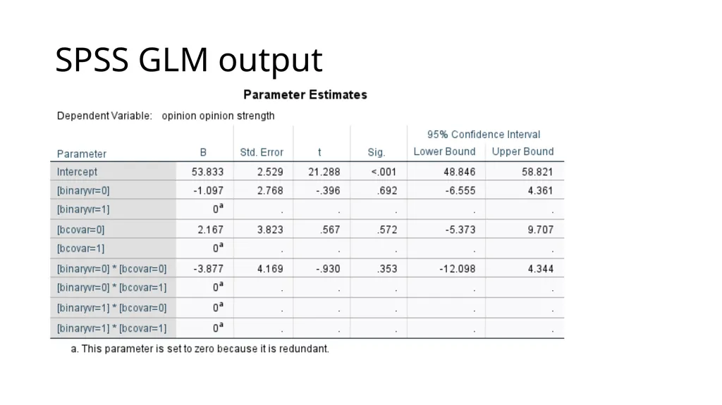
In the table of Parameter Estimates, we find the unstandardized coefficients (called B) and their standard errors, the t test statistics, the p-values (in the column Sig.) and the 95% CIs.<br>
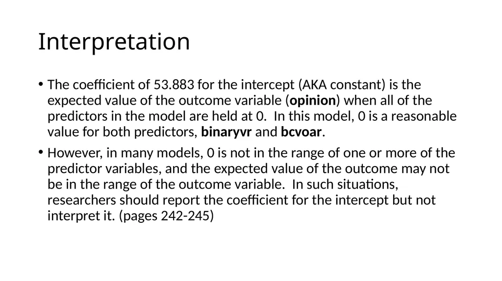
slide24. Interpretation The coefficient of 53.883 for the intercept (AKA constant) is the expected value of the outcome variable (opinion) when all of the predictors in the model are held at 0. In this model, 0 is a reasonable value for both predictors, binaryvr and bcvoar.
However, in many models, 0 is not in the range of one or more of the predictor variables, and the expected value of the outcome may not be in the range of the outcome variable. In such situations, researchers should report the coefficient for the intercept but not interpret it. (pages 242-245)<br>
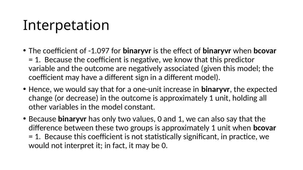
slide25. Interpetation The coefficient of -1.097 for binaryvr is the effect of binaryvr when bcovar = 1. Because the coefficient is negative, we know that this predictor variable and the outcome are negatively associated (given this model; the coefficient may have a different sign in a different model).
Hence, we would say that for a one-unit increase in binaryvr, the expected change (or decrease) in the outcome is approximately 1 unit, holding all other variables in the model constant.
Because binaryvr has only two values, 0 and 1, we can also say that the difference between these two groups is approximately 1 unit when bcovar = 1. Because this coefficient is not statistically significant, in practice, we would not interpret it; in fact, it may be 0.<br>
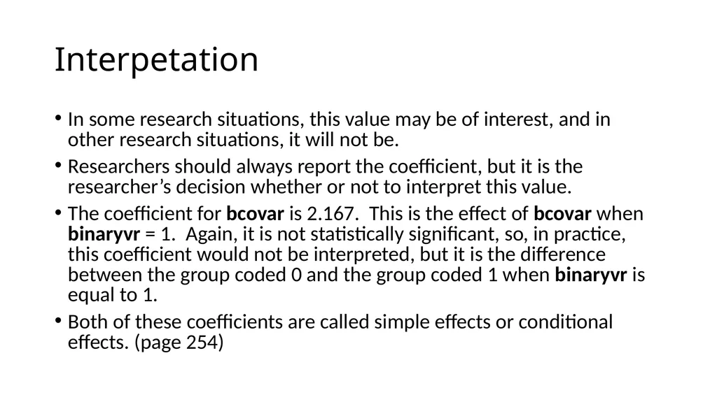
slide26. Interpetation In some research situations, this value may be of interest, and in other research situations, it will not be.
Researchers should always report the coefficient, but it is the researcher’s decision whether or not to interpret this value.
The coefficient for bcovar is 2.167. This is the effect of bcovar when binaryvr = 1. Again, it is not statistically significant, so, in practice, this coefficient would not be interpreted, but it is the difference between the group coded 0 and the group coded 1 when binaryvr is equal to 1.
Both of these coefficients are called simple effects or conditional effects. (page 254)<br>
slide27. Caution! Remember that these coefficients are simple effects.
When writing about these lower-order terms, the phrases “main effects” and “average effects” should be avoided.
NOTE: The term “main effect” comes from ANOVA. It is used because the coding of the lower-order effects is different in ANOVA than in regression.<br>
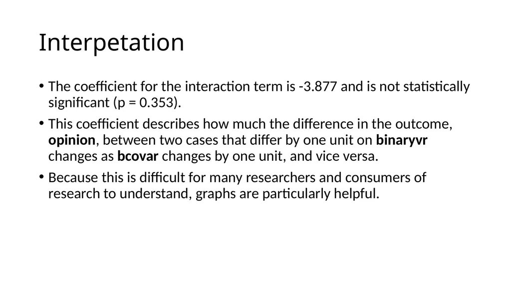
slide28. Interpetation The coefficient for the interaction term is -3.877 and is not statistically significant (p = 0.353).
This coefficient describes how much the difference in the outcome, opinion, between two cases that differ by one unit on binaryvr changes as bcovar changes by one unit, and vice versa.
Because this is difficult for many researchers and consumers of research to understand, graphs are particularly helpful.<br>
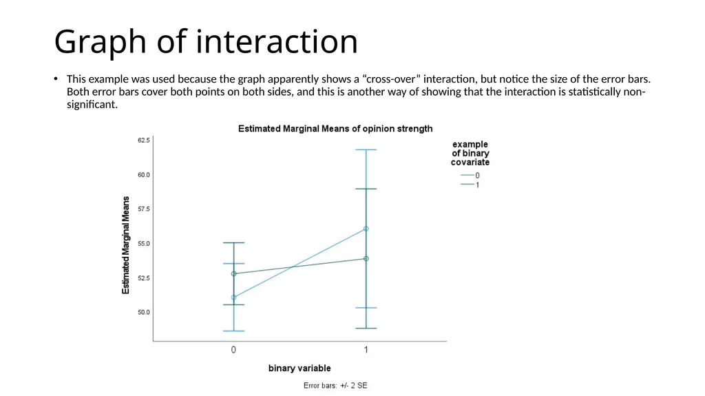
slide29. Graph of interaction This example was used because the graph apparently shows a “cross-over” interaction, but notice the size of the error bars. Both error bars cover both points on both sides, and this is another way of showing that the interaction is statistically non-significant.<br>
slide30. Try it yourself What is the difference between a dichotomous variable and a binary variable?
Why would this matter in a regression analysis?
Given that the interaction term is not statistically significant, should the interaction term remain in the model or be removed?<br>
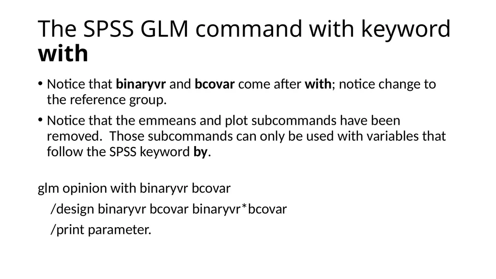
slide31. The SPSS GLM command with keyword with Notice that binaryvr and bcovar come after with; notice change to the reference group.
Notice that the emmeans and plot subcommands have been removed. Those subcommands can only be used with variables that follow the SPSS keyword by.
glm opinion with binaryvr bcovar
/design binaryvr bcovar binaryvr*bcovar
/print parameter.<br>
slide32. SPSS GLM output using the keyword with<br>
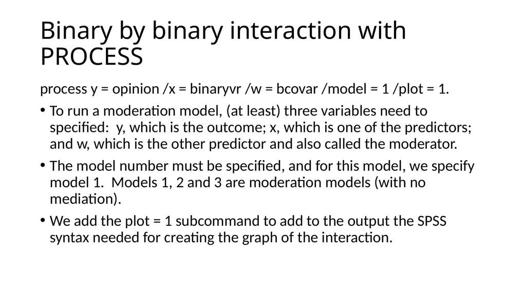
slide33. Binary by binary interaction with PROCESS process y = opinion /x = binaryvr /w = bcovar /model = 1 /plot = 1.
To run a moderation model, (at least) three variables need to specified: y, which is the outcome; x, which is one of the predictors; and w, which is the other predictor and also called the moderator.
The model number must be specified, and for this model, we specify model 1. Models 1, 2 and 3 are moderation models (with no mediation).
We add the plot = 1 subcommand to add to the output the SPSS syntax needed for creating the graph of the interaction.<br>
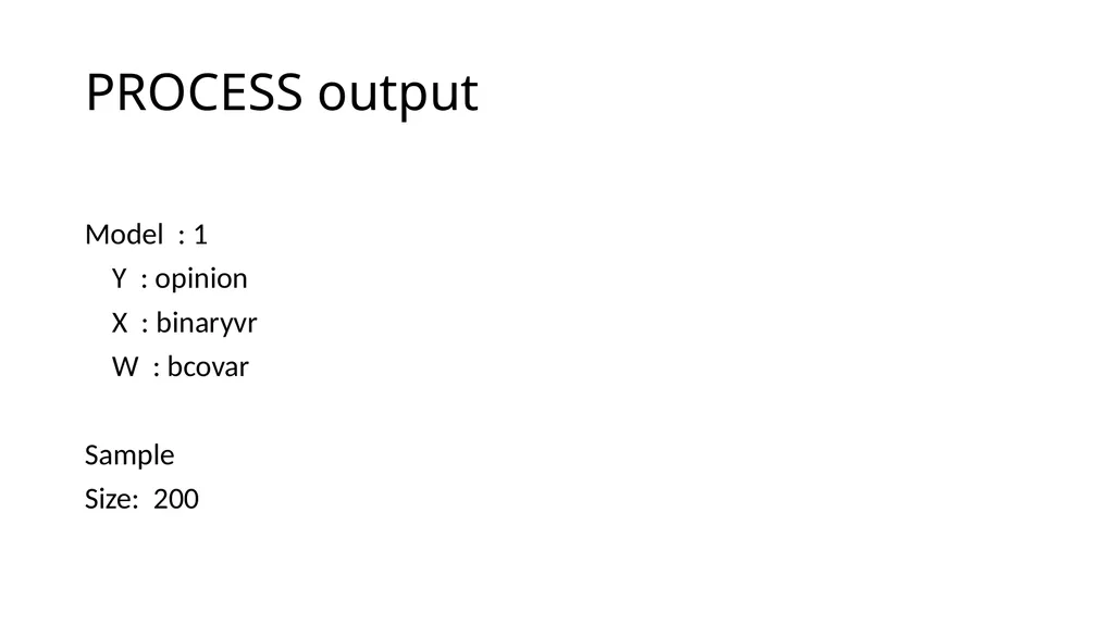
slide34. PROCESS output Model : 1
Y : opinion
X : binaryvr
W : bcovar

Sample
Size: 200<br>
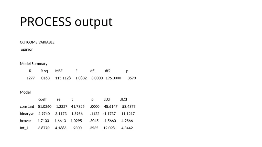
slide35. PROCESS output OUTCOME VARIABLE:
opinion

Model Summary
R R-sq MSE F df1 df2 p
.1277 .0163 115.1128 1.0832 3.0000 196.0000 .3573

Model
coeff se t p LLCI ULCI
constant 51.0260 1.2227 41.7325 .0000 48.6147 53.4373
binaryvr 4.9740 3.1173 1.5956 .1122 -1.1737 11.1217
bcovar 1.7103 1.6613 1.0295 .3045 -1.5660 4.9866
Int_1 -3.8770 4.1686 -.9300 .3535 -12.0981 4.3442<br>
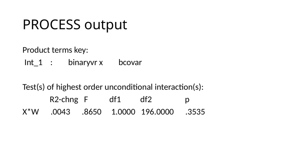
slide36. PROCESS output Product terms key:
Int_1 : binaryvr x bcovar

Test(s) of highest order unconditional interaction(s):
R2-chng F df1 df2 p
X*W .0043 .8650 1.0000 196.0000 .3535<br>
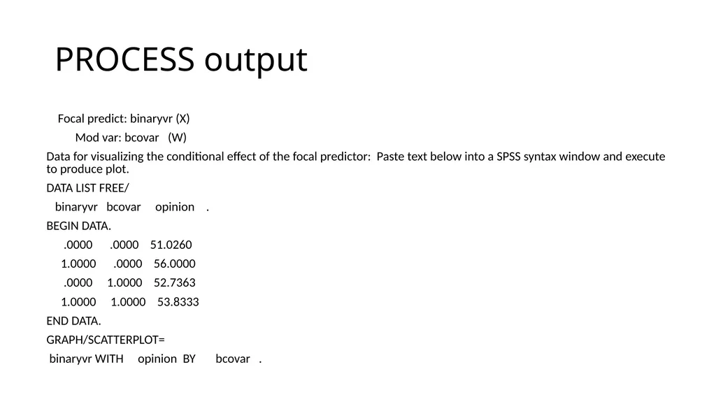
slide37. PROCESS output Focal predict: binaryvr (X)
Mod var: bcovar (W)
Data for visualizing the conditional effect of the focal predictor: Paste text below into a SPSS syntax window and execute to produce plot.
DATA LIST FREE/
binaryvr bcovar opinion .
BEGIN DATA.
.0000 .0000 51.0260
1.0000 .0000 56.0000
.0000 1.0000 52.7363
1.0000 1.0000 53.8333
END DATA.
GRAPH/SCATTERPLOT=
binaryvr WITH opinion BY bcovar .<br>
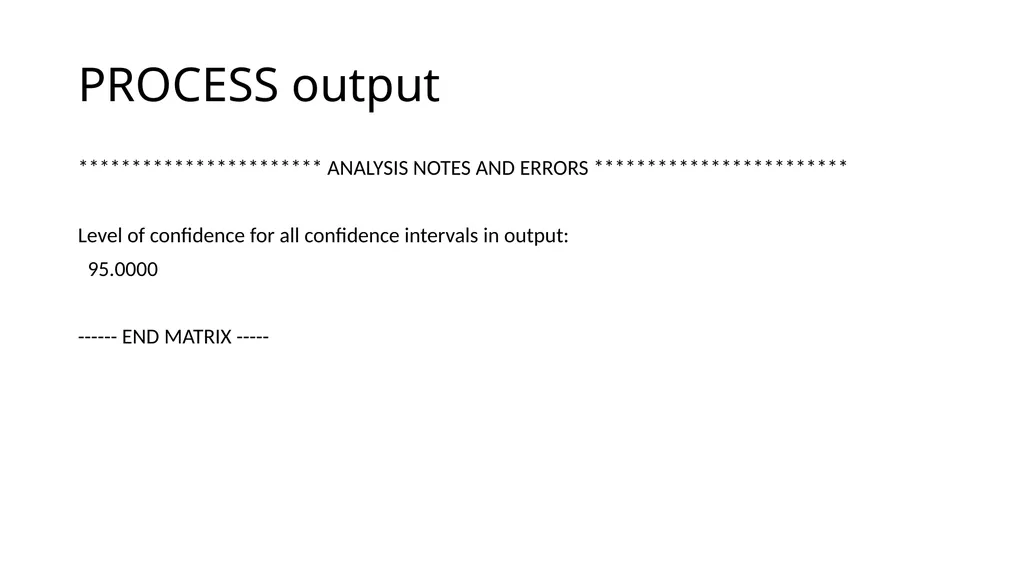
slide38. PROCESS output *********************** ANALYSIS NOTES AND ERRORS ************************

Level of confidence for all confidence intervals in output:
95.0000

------ END MATRIX -----<br>
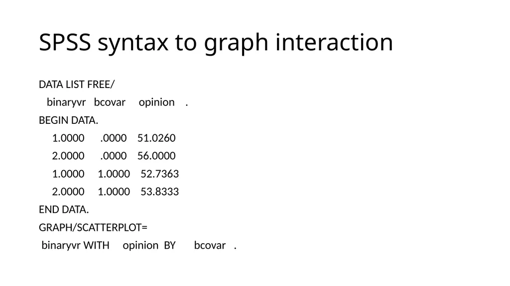
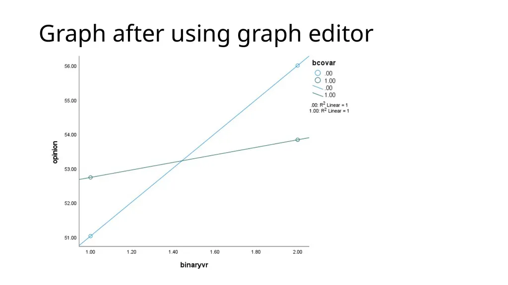
slide39. SPSS syntax to graph interaction DATA LIST FREE/
binaryvr bcovar opinion .
BEGIN DATA.
1.0000 .0000 51.0260
2.0000 .0000 56.0000
1.0000 1.0000 52.7363
2.0000 1.0000 53.8333
END DATA.
GRAPH/SCATTERPLOT=
binaryvr WITH opinion BY bcovar .<br>
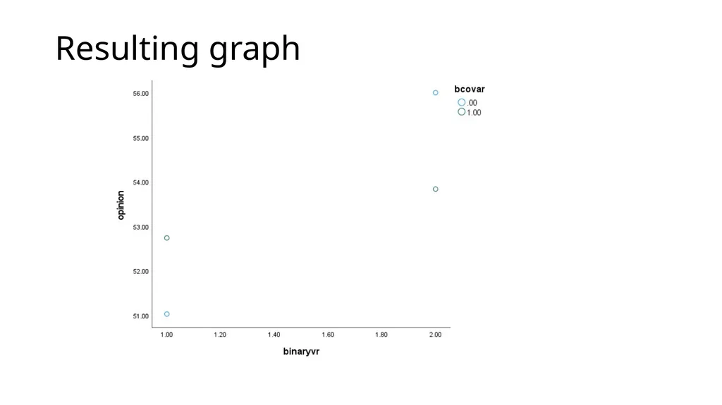
slide40. Resulting graph<br>
slide41. Graph after using graph editor<br>
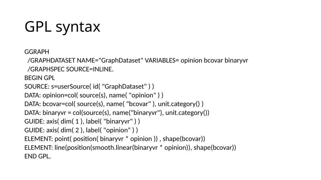
slide42. GPL syntax GGRAPH
/GRAPHDATASET NAME="GraphDataset" VARIABLES= opinion bcovar binaryvr
/GRAPHSPEC SOURCE=INLINE.
BEGIN GPL
SOURCE: s=userSource( id( "GraphDataset" ) )
DATA: opinion=col( source(s), name( "opinion" ) )
DATA: bcovar=col( source(s), name( "bcovar" ), unit.category() )
DATA: binaryvr = col(source(s), name("binaryvr"), unit.category())
GUIDE: axis( dim( 1 ), label( "binaryvr" ) )
GUIDE: axis( dim( 2 ), label( "opinion" ) )
ELEMENT: point( position( binaryvr * opinion )) , shape(bcovar))
ELEMENT: line(position(smooth.linear(binaryvr * opinion)), shape(bcovar))
END GPL.<br>
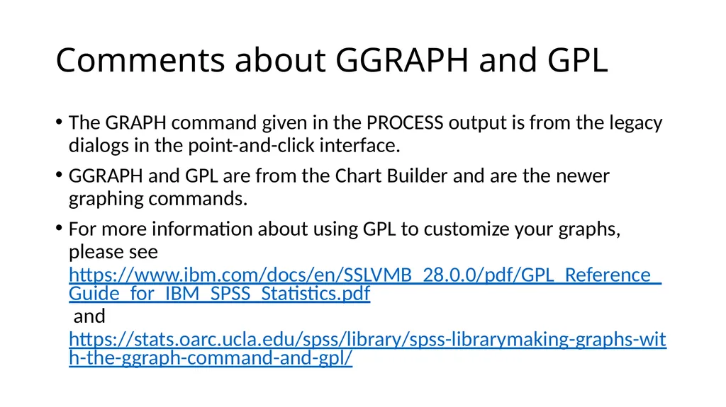
slide43. Comments about GGRAPH and GPL The GRAPH command given in the PROCESS output is from the legacy dialogs in the point-and-click interface.
GGRAPH and GPL are from the Chart Builder and are the newer graphing commands.
For more information about using GPL to customize your graphs, please see https://www.ibm.com/docs/en/SSLVMB_28.0.0/pdf/GPL_Reference_Guide_for_IBM_SPSS_Statistics.pdf and https://stats.oarc.ucla.edu/spss/library/spss-librarymaking-graphs-with-the-ggraph-command-and-gpl/<br>
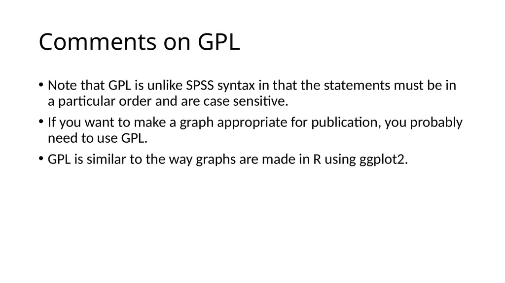
slide44. Comments on GPL Note that GPL is unlike SPSS syntax in that the statements must be in a particular order and are case sensitive.
If you want to make a graph appropriate for publication, you probably need to use GPL.
GPL is similar to the way graphs are made in R using ggplot2.<br>
slide45. Binary by three-level interaction<br>
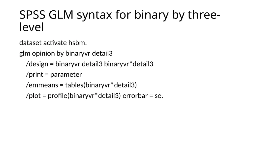
slide46. SPSS GLM syntax for binary by three-level dataset activate hsbm.
glm opinion by binaryvr detail3
/design = binaryvr detail3 binaryvr*detail3
/print = parameter
/emmeans = tables(binaryvr*detail3)
/plot = profile(binaryvr*detail3) errorbar = se.<br>
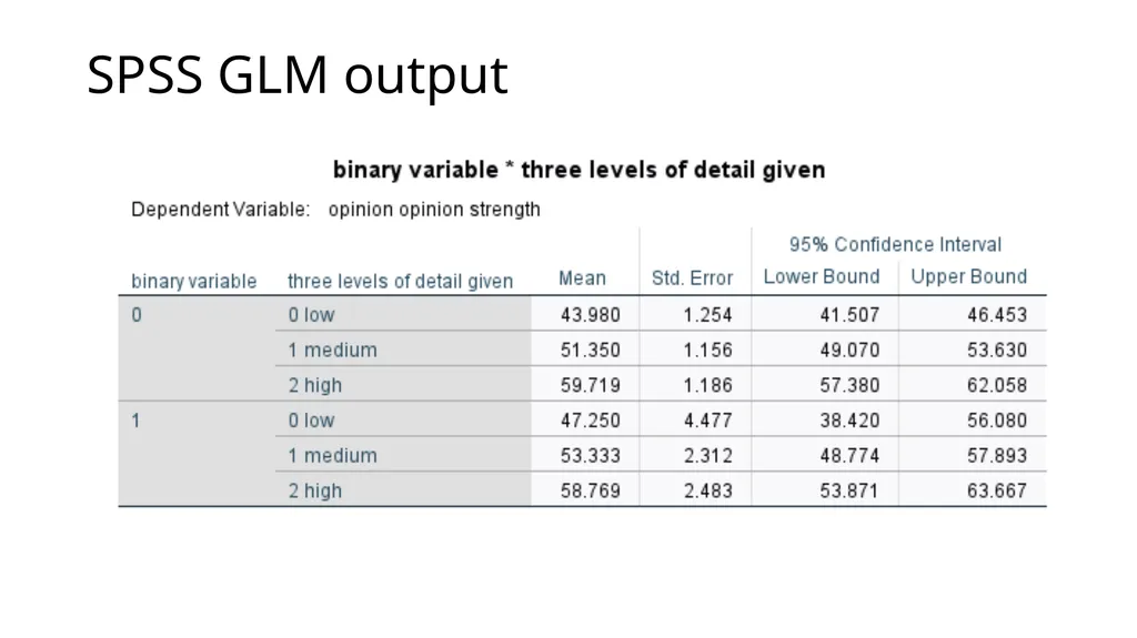
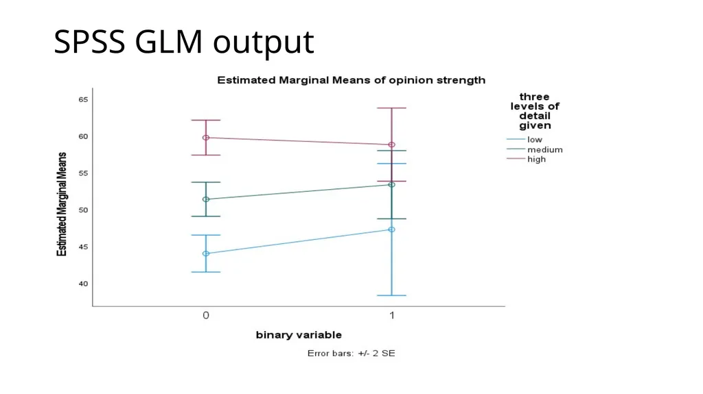
slide47. SPSS GLM output<br>
slide48. SPSS GLM output<br>
slide49. SPSS GLM output<br>
slide50. SPSS GLM output<br>
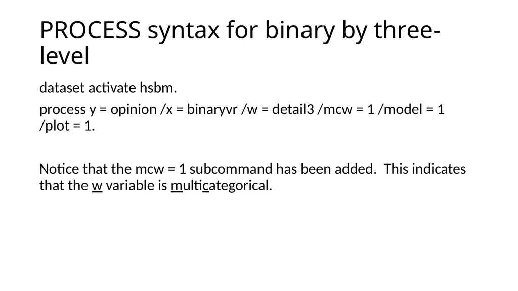
slide51. PROCESS syntax for binary by three-level dataset activate hsbm.
process y = opinion /x = binaryvr /w = detail3 /mcw = 1 /model = 1 /plot = 1.

Notice that the mcw = 1 subcommand has been added. This indicates that the w variable is multicategorical.<br>
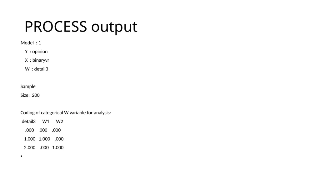
slide52. PROCESS output Model : 1
Y : opinion
X : binaryvr
W : detail3

Sample
Size: 200

Coding of categorical W variable for analysis:
detail3 W1 W2
.000 .000 .000
1.000 1.000 .000
2.000 .000 1.000<br>
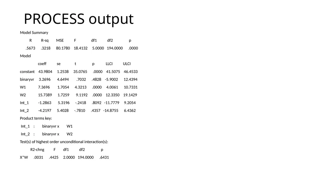
slide53. PROCESS output Model Summary
R R-sq MSE F df1 df2 p
.5673 .3218 80.1780 18.4132 5.0000 194.0000 .0000
Model
coeff se t p LLCI ULCI
constant 43.9804 1.2538 35.0765 .0000 41.5075 46.4533
binaryvr 3.2696 4.6494 .7032 .4828 -5.9002 12.4394
W1 7.3696 1.7054 4.3213 .0000 4.0061 10.7331
W2 15.7389 1.7259 9.1192 .0000 12.3350 19.1429
Int_1 -1.2863 5.3196 -.2418 .8092 -11.7779 9.2054
Int_2 -4.2197 5.4028 -.7810 .4357 -14.8755 6.4362
Product terms key:
Int_1 : binaryvr x W1
Int_2 : binaryvr x W2
Test(s) of highest order unconditional interaction(s):
R2-chng F df1 df2 p
X*W .0031 .4425 2.0000 194.0000 .6431<br>
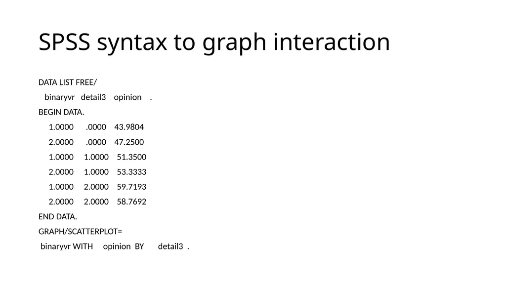
slide54. SPSS syntax to graph interaction DATA LIST FREE/
binaryvr detail3 opinion .
BEGIN DATA.
1.0000 .0000 43.9804
2.0000 .0000 47.2500
1.0000 1.0000 51.3500
2.0000 1.0000 53.3333
1.0000 2.0000 59.7193
2.0000 2.0000 58.7692
END DATA.
GRAPH/SCATTERPLOT=
binaryvr WITH opinion BY detail3 .<br>
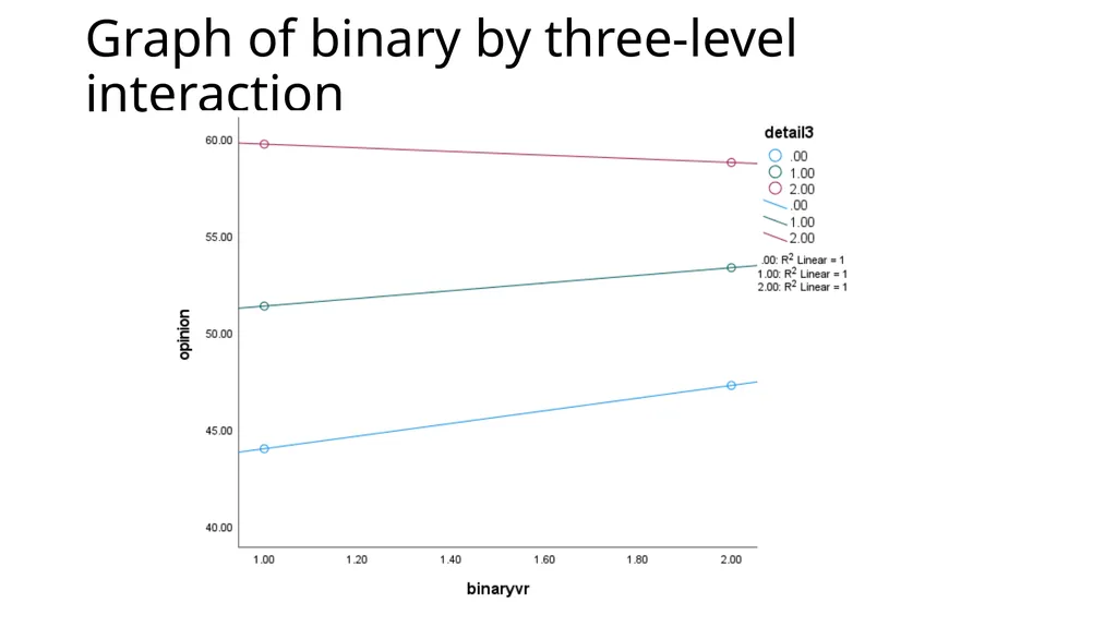
slide55. Graph of binary by three-level interaction<br>
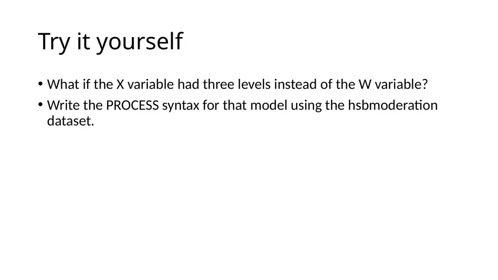
slide56. Try it yourself What if the X variable had three levels instead of the W variable?
Write the PROCESS syntax for that model using the hsbmoderation dataset.<br>
slide57. Binary by continuous interaction<br>
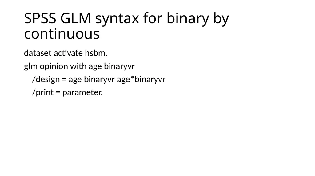
slide58. SPSS GLM syntax for binary by continuous dataset activate hsbm.
glm opinion with age binaryvr
/design = age binaryvr age*binaryvr
/print = parameter.<br>
slide59. SPSS GLM output<br>
slide60. SPSS GLM output<br>
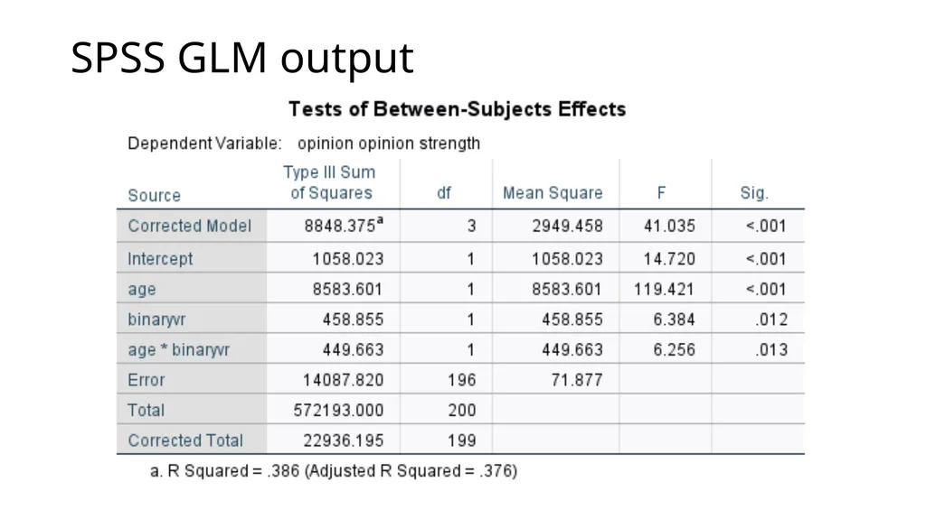
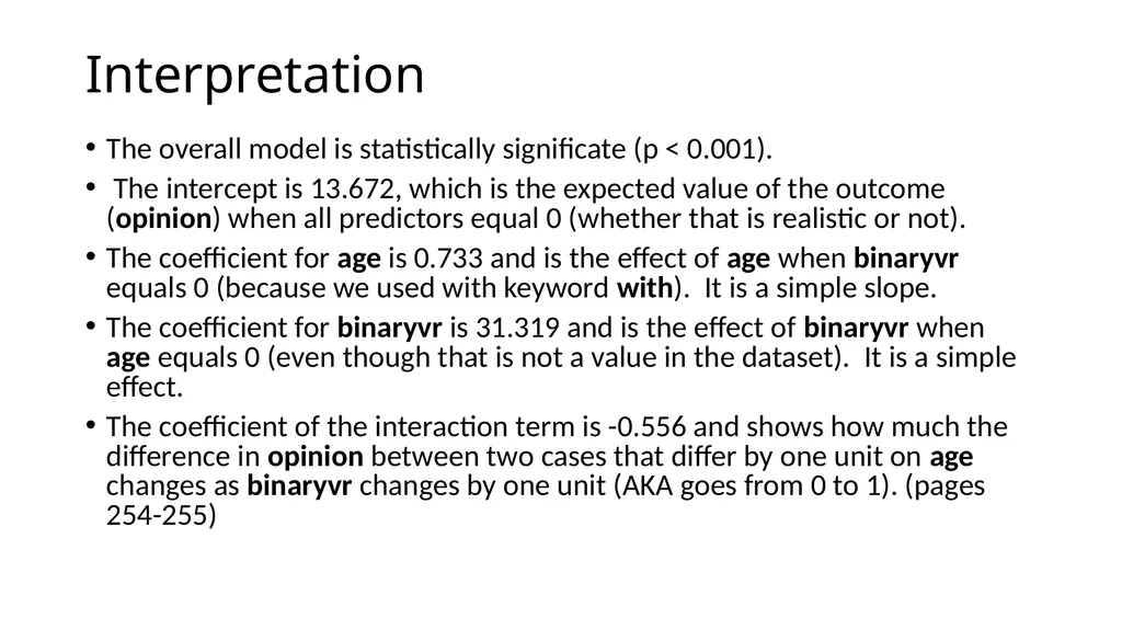
slide61. Interpretation The overall model is statistically significate (p < 0.001).
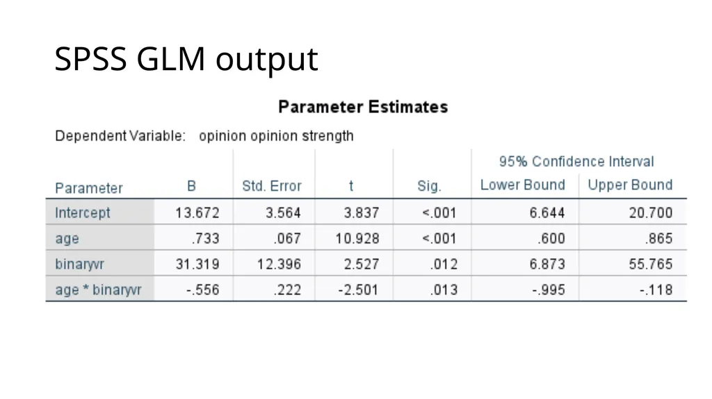
The intercept is 13.672, which is the expected value of the outcome (opinion) when all predictors equal 0 (whether that is realistic or not).
The coefficient for age is 0.733 and is the effect of age when binaryvr equals 0 (because we used with keyword with). It is a simple slope.
The coefficient for binaryvr is 31.319 and is the effect of binaryvr when age equals 0 (even though that is not a value in the dataset). It is a simple effect.
The coefficient of the interaction term is -0.556 and shows how much the difference in opinion between two cases that differ by one unit on age changes as binaryvr changes by one unit (AKA goes from 0 to 1). (pages 254-255)<br>
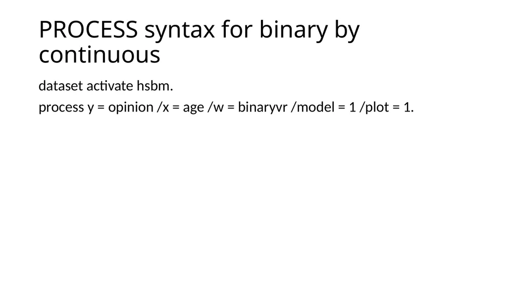
slide62. PROCESS syntax for binary by continuous dataset activate hsbm.
process y = opinion /x = age /w = binaryvr /model = 1 /plot = 1.<br>
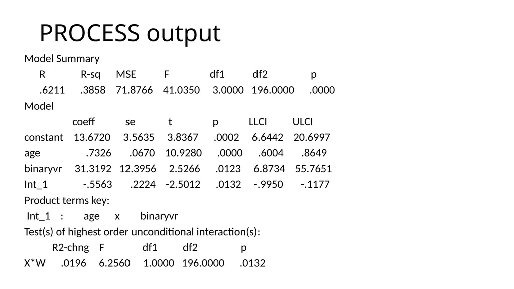
slide63. PROCESS output Model Summary
R R-sq MSE F df1 df2 p
.6211 .3858 71.8766 41.0350 3.0000 196.0000 .0000
Model
coeff se t p LLCI ULCI
constant 13.6720 3.5635 3.8367 .0002 6.6442 20.6997
age .7326 .0670 10.9280 .0000 .6004 .8649
binaryvr 31.3192 12.3956 2.5266 .0123 6.8734 55.7651
Int_1 -.5563 .2224 -2.5012 .0132 -.9950 -.1177
Product terms key:
Int_1 : age x binaryvr
Test(s) of highest order unconditional interaction(s):
R2-chng F df1 df2 p
X*W .0196 6.2560 1.0000 196.0000 .0132<br>
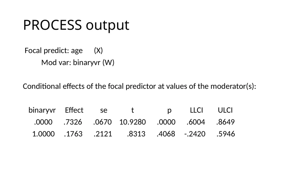
slide64. PROCESS output Focal predict: age (X)
Mod var: binaryvr (W)

Conditional effects of the focal predictor at values of the moderator(s):

binaryvr Effect se t p LLCI ULCI
.0000 .7326 .0670 10.9280 .0000 .6004 .8649
1.0000 .1763 .2121 .8313 .4068 -.2420 .5946<br>
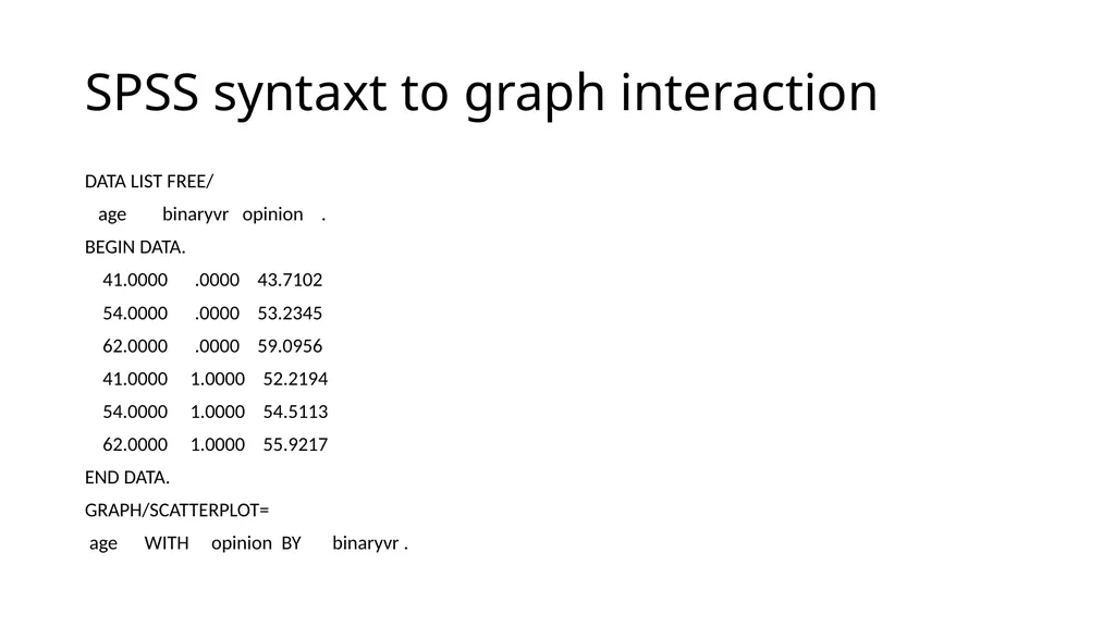
slide65. SPSS syntaxt to graph interaction DATA LIST FREE/
age binaryvr opinion .
BEGIN DATA.
41.0000 .0000 43.7102
54.0000 .0000 53.2345
62.0000 .0000 59.0956
41.0000 1.0000 52.2194
54.0000 1.0000 54.5113
62.0000 1.0000 55.9217
END DATA.
GRAPH/SCATTERPLOT=
age WITH opinion BY binaryvr .<br>
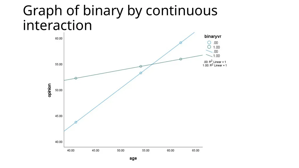
slide66. Graph of binary by continuous interaction<br>
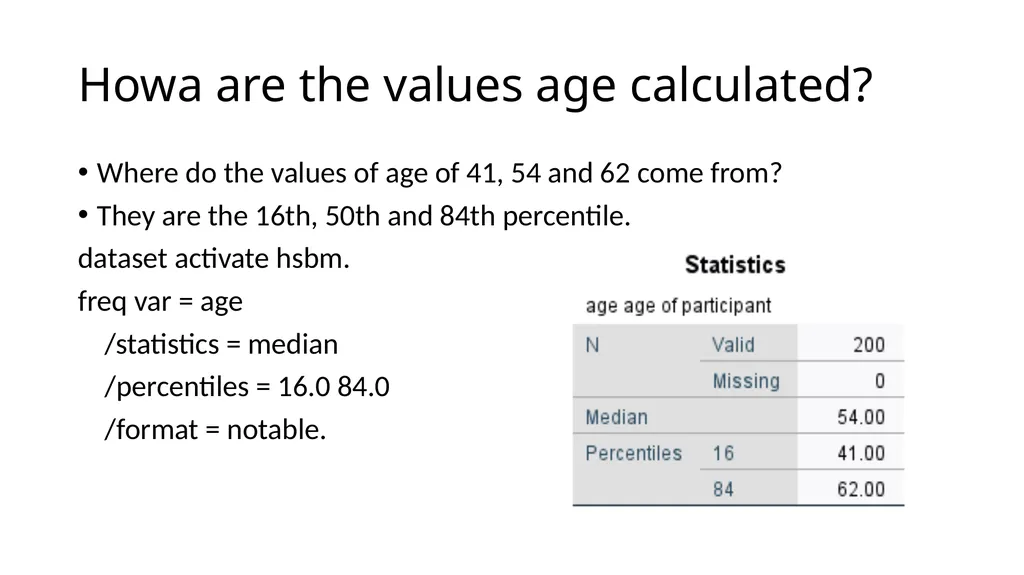
slide67. Howa are the values age calculated? Where do the values of age of 41, 54 and 62 come from?
They are the 16th, 50th and 84th percentile.
dataset activate hsbm.
freq var = age
/statistics = median
/percentiles = 16.0 84.0
/format = notable.<br>
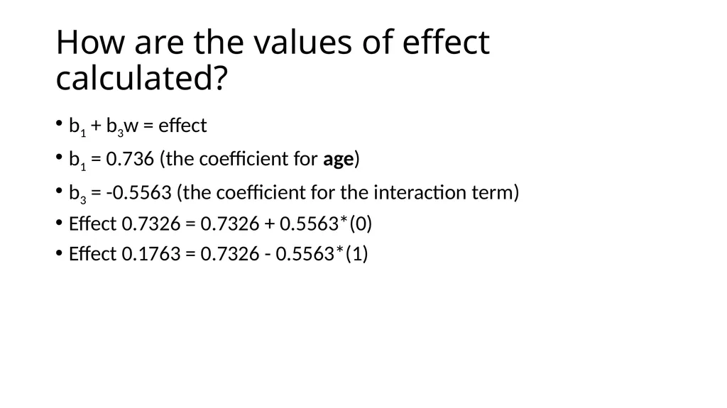
slide68. How are the values of effect calculated? b1 + b3w = effect
b1 = 0.736 (the coefficient for age)
b3 = -0.5563 (the coefficient for the interaction term)
Effect 0.7326 = 0.7326 + 0.5563*(0)
Effect 0.1763 = 0.7326 - 0.5563*(1)<br>
slide69. Continuous by three-level interaction<br>
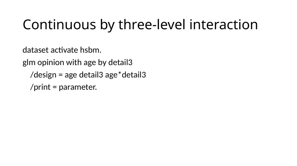
slide70. Continuous by three-level interaction dataset activate hsbm.
glm opinion with age by detail3
/design = age detail3 age*detail3
/print = parameter.<br>
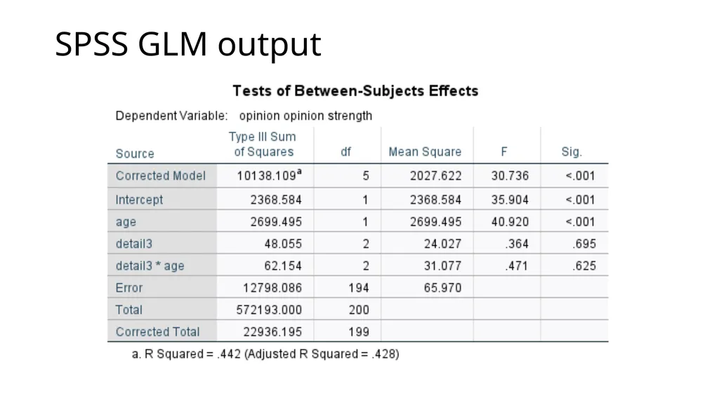
slide71. SPSS GLM output<br>
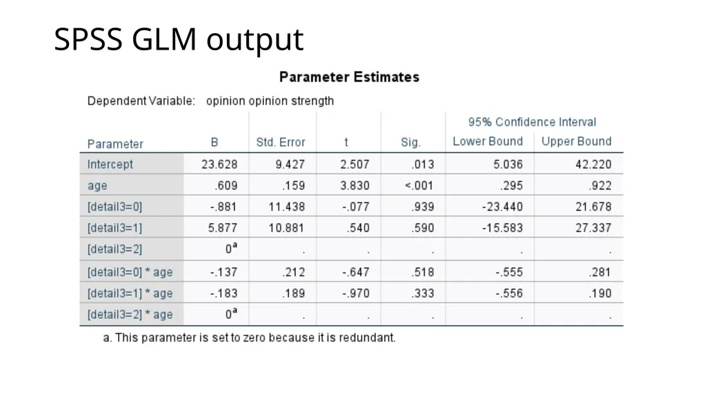
slide72. SPSS GLM output<br>
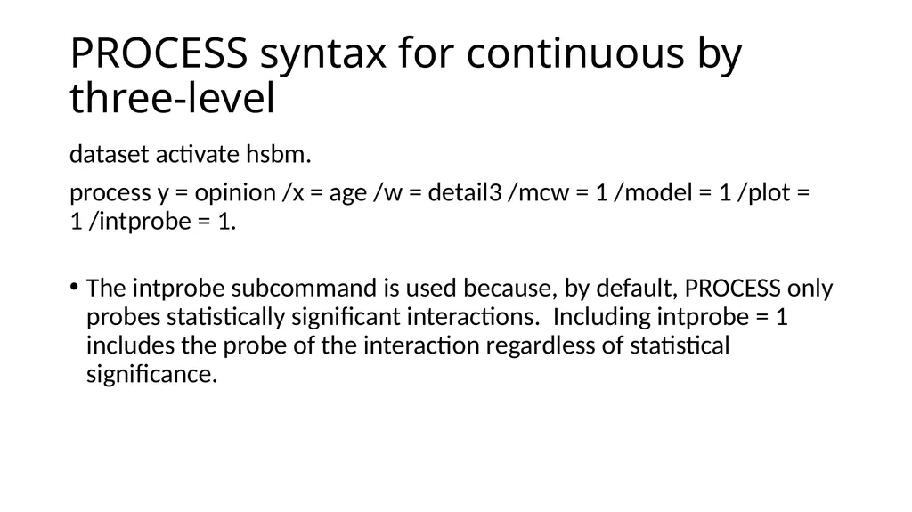
slide73. PROCESS syntax for continuous by three-level dataset activate hsbm.
process y = opinion /x = age /w = detail3 /mcw = 1 /model = 1 /plot = 1 /intprobe = 1. 
The intprobe subcommand is used because, by default, PROCESS only probes statistically significant interactions. Including intprobe = 1 includes the probe of the interaction regardless of statistical significance.<br>
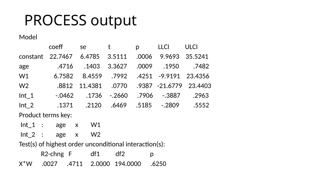
slide74. PROCESS output Model
coeff se t p LLCI ULCI
constant 22.7467 6.4785 3.5111 .0006 9.9693 35.5241
age .4716 .1403 3.3627 .0009 .1950 .7482
W1 6.7582 8.4559 .7992 .4251 -9.9191 23.4356
W2 .8812 11.4381 .0770 .9387 -21.6779 23.4403
Int_1 -.0462 .1736 -.2660 .7906 -.3887 .2963
Int_2 .1371 .2120 .6469 .5185 -.2809 .5552
Product terms key:
Int_1 : age x W1
Int_2 : age x W2
Test(s) of highest order unconditional interaction(s):
R2-chng F df1 df2 p
X*W .0027 .4711 2.0000 194.0000 .6250<br>
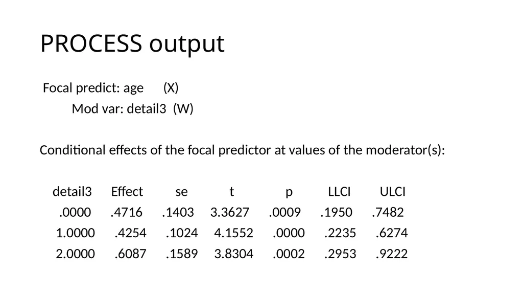
slide75. PROCESS output Focal predict: age (X)
Mod var: detail3 (W)

Conditional effects of the focal predictor at values of the moderator(s):

detail3 Effect se t p LLCI ULCI
.0000 .4716 .1403 3.3627 .0009 .1950 .7482
1.0000 .4254 .1024 4.1552 .0000 .2235 .6274
2.0000 .6087 .1589 3.8304 .0002 .2953 .9222<br>
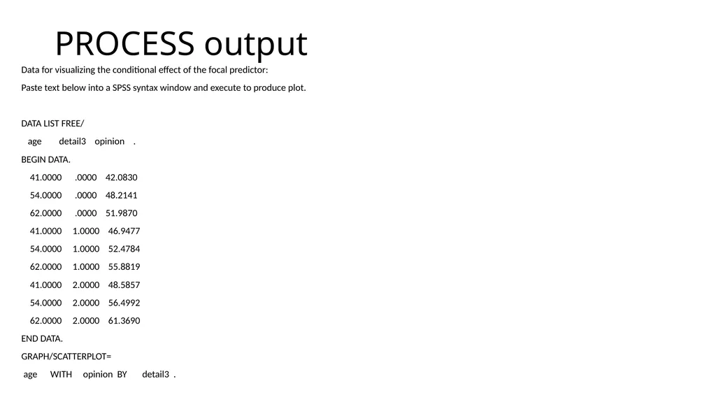
slide76. PROCESS output Data for visualizing the conditional effect of the focal predictor:
Paste text below into a SPSS syntax window and execute to produce plot.

DATA LIST FREE/
age detail3 opinion .
BEGIN DATA.
41.0000 .0000 42.0830
54.0000 .0000 48.2141
62.0000 .0000 51.9870
41.0000 1.0000 46.9477
54.0000 1.0000 52.4784
62.0000 1.0000 55.8819
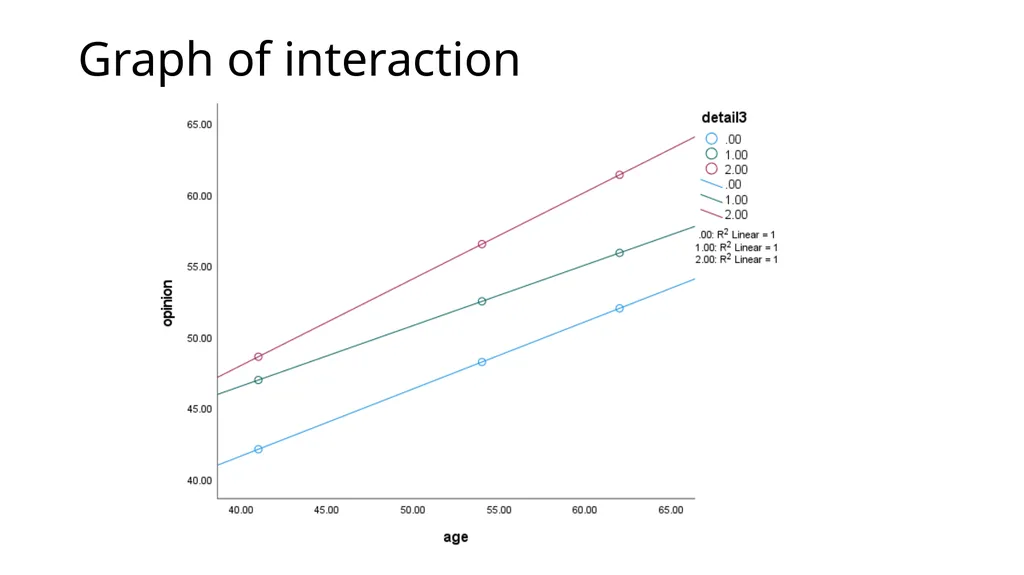
41.0000 2.0000 48.5857
54.0000 2.0000 56.4992
62.0000 2.0000 61.3690
END DATA.
GRAPH/SCATTERPLOT=
age WITH opinion BY detail3 .<br>
slide77. Graph of interaction<br>
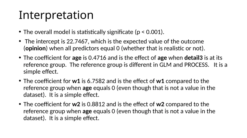
slide78. Interpretation The overall model is statistically significate (p < 0.001).
The intercept is 22.7467, which is the expected value of the outcome (opinion) when all predictors equal 0 (whether that is realistic or not).
The coefficient for age is 0.4716 and is the effect of age when detail3 is at its reference group. The reference group is different in GLM and PROCESS. It is a simple effect.
The coefficient for w1 is 6.7582 and is the effect of w1 compared to the reference group when age equals 0 (even though that is not a value in the dataset). It is a simple effect.
The coefficient for w2 is 0.8812 and is the effect of w2 compared to the reference group when age equals 0 (even though that is not a value in the dataset). It is a simple effect.<br>
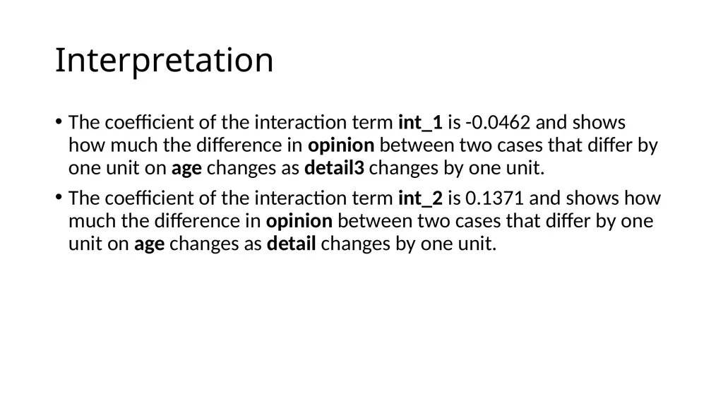
slide79. Interpretation The coefficient of the interaction term int_1 is -0.0462 and shows how much the difference in opinion between two cases that differ by one unit on age changes as detail3 changes by one unit.
The coefficient of the interaction term int_2 is 0.1371 and shows how much the difference in opinion between two cases that differ by one unit on age changes as detail changes by one unit.<br>
slide80. Contiuous by continuous interaction<br>
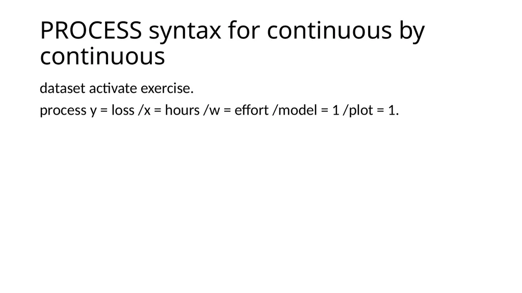
slide81. PROCESS syntax for continuous by continuous dataset activate exercise.
process y = loss /x = hours /w = effort /model = 1 /plot = 1.<br>
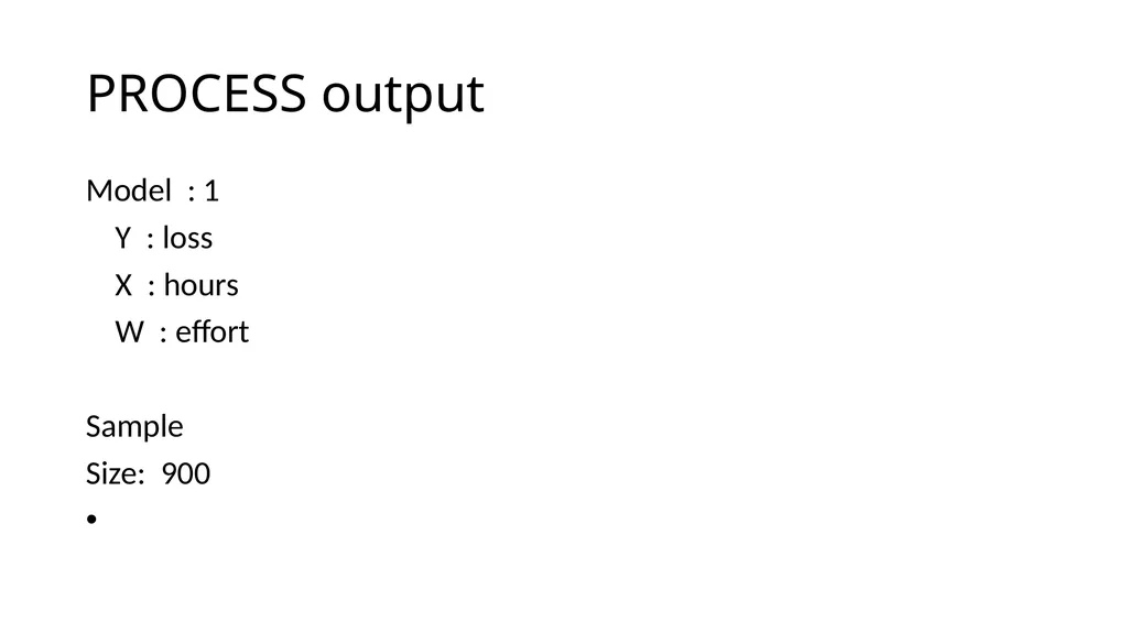
slide82. PROCESS output Model : 1
Y : loss
X : hours
W : effort

Sample
Size: 900<br>
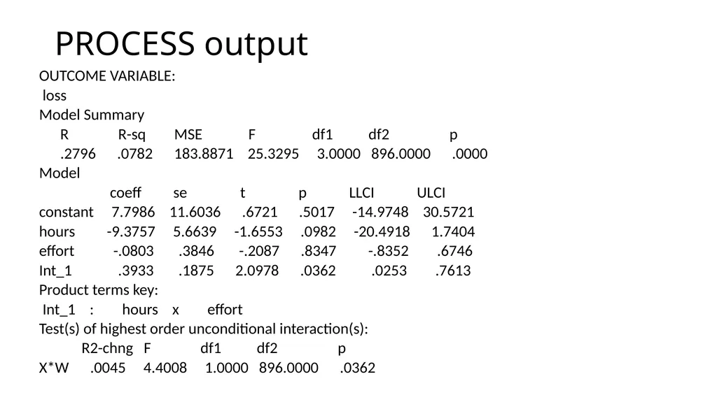
slide83. PROCESS output OUTCOME VARIABLE:
loss
Model Summary
R R-sq MSE F df1 df2 p
.2796 .0782 183.8871 25.3295 3.0000 896.0000 .0000
Model
coeff se t p LLCI ULCI
constant 7.7986 11.6036 .6721 .5017 -14.9748 30.5721
hours -9.3757 5.6639 -1.6553 .0982 -20.4918 1.7404
effort -.0803 .3846 -.2087 .8347 -.8352 .6746
Int_1 .3933 .1875 2.0978 .0362 .0253 .7613
Product terms key:
Int_1 : hours x effort
Test(s) of highest order unconditional interaction(s):
R2-chng F df1 df2 p
X*W .0045 4.4008 1.0000 896.0000 .0362<br>
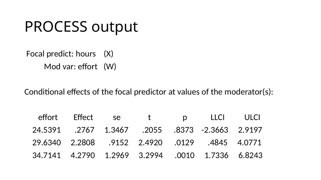
slide84. PROCESS output Focal predict: hours (X)
Mod var: effort (W)

Conditional effects of the focal predictor at values of the moderator(s):

effort Effect se t p LLCI ULCI
24.5391 .2767 1.3467 .2055 .8373 -2.3663 2.9197
29.6340 2.2808 .9152 2.4920 .0129 .4845 4.0771
34.7141 4.2790 1.2969 3.2994 .0010 1.7336 6.8243<br>
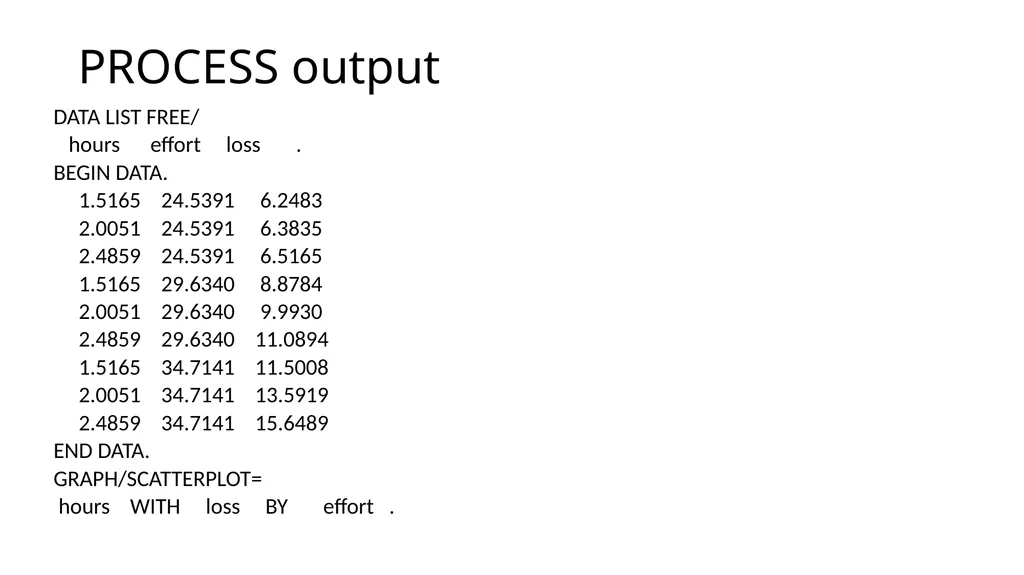
slide85. PROCESS output DATA LIST FREE/
hours effort loss .
BEGIN DATA.
1.5165 24.5391 6.2483
2.0051 24.5391 6.3835
2.4859 24.5391 6.5165
1.5165 29.6340 8.8784
2.0051 29.6340 9.9930
2.4859 29.6340 11.0894
1.5165 34.7141 11.5008
2.0051 34.7141 13.5919
2.4859 34.7141 15.6489
END DATA.
GRAPH/SCATTERPLOT=
hours WITH loss BY effort .<br>
slide86. PROCESS output Level of confidence for all confidence intervals in output:
95.0000

W values in conditional tables are the 16th, 50th, and 84th percentiles.<br>
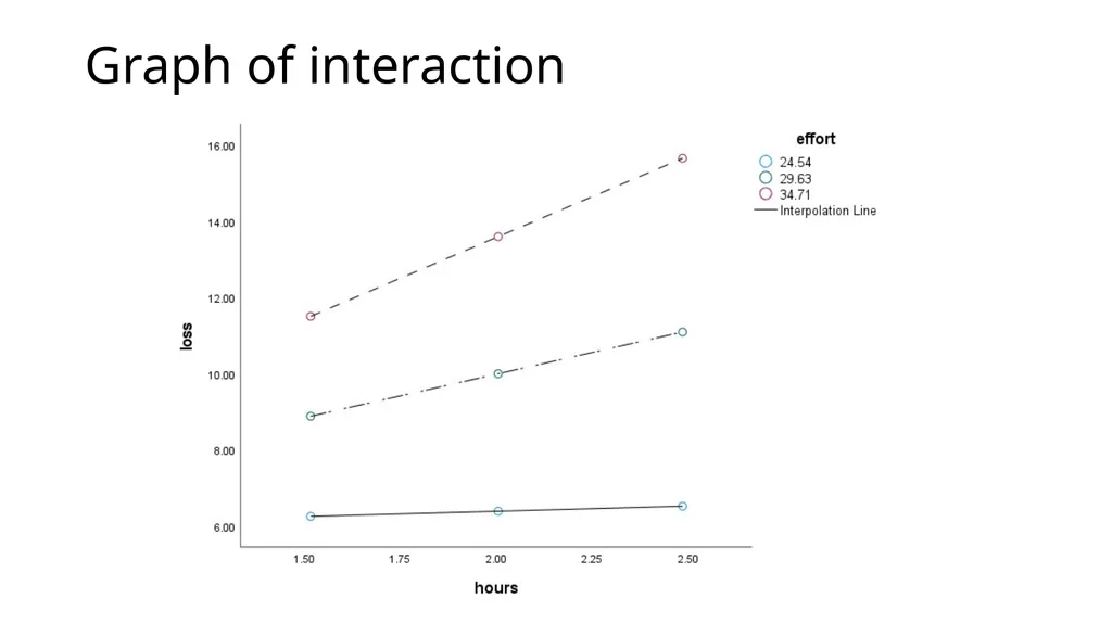
slide87. Graph of interaction<br>
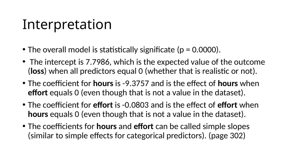
slide88. Interpretation The overall model is statistically significate (p = 0.0000).
The intercept is 7.7986, which is the expected value of the outcome (loss) when all predictors equal 0 (whether that is realistic or not).
The coefficient for hours is -9.3757 and is the effect of hours when effort equals 0 (even though that is not a value in the dataset).
The coefficient for effort is -0.0803 and is the effect of effort when hours equals 0 (even though that is not a value in the dataset).
The coefficients for hours and effort can be called simple slopes (similar to simple effects for categorical predictors). (page 302)<br>
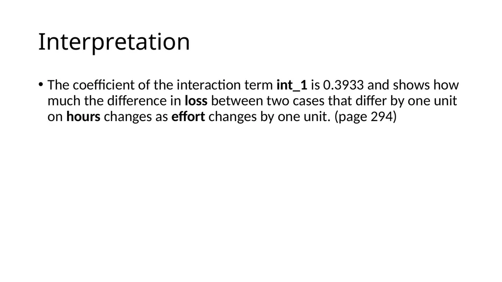
slide89. Interpretation The coefficient of the interaction term int_1 is 0.3933 and shows how much the difference in loss between two cases that differ by one unit on hours changes as effort changes by one unit. (page 294)<br>
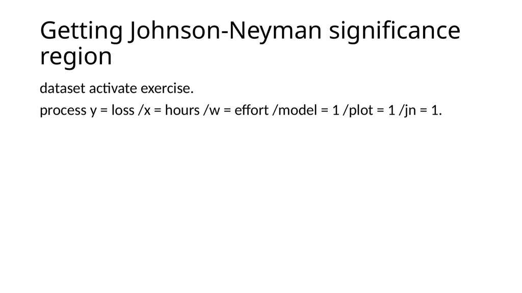
slide90. Getting Johnson-Neyman significance region dataset activate exercise.
process y = loss /x = hours /w = effort /model = 1 /plot = 1 /jn = 1.<br>
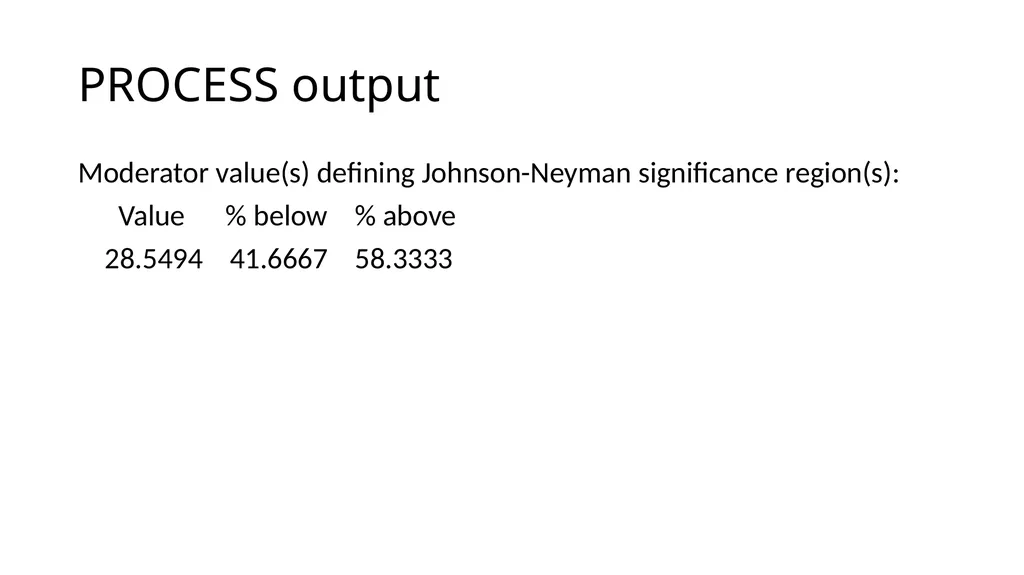
slide91. PROCESS output Moderator value(s) defining Johnson-Neyman significance region(s):
Value % below % above
28.5494 41.6667 58.3333<br>
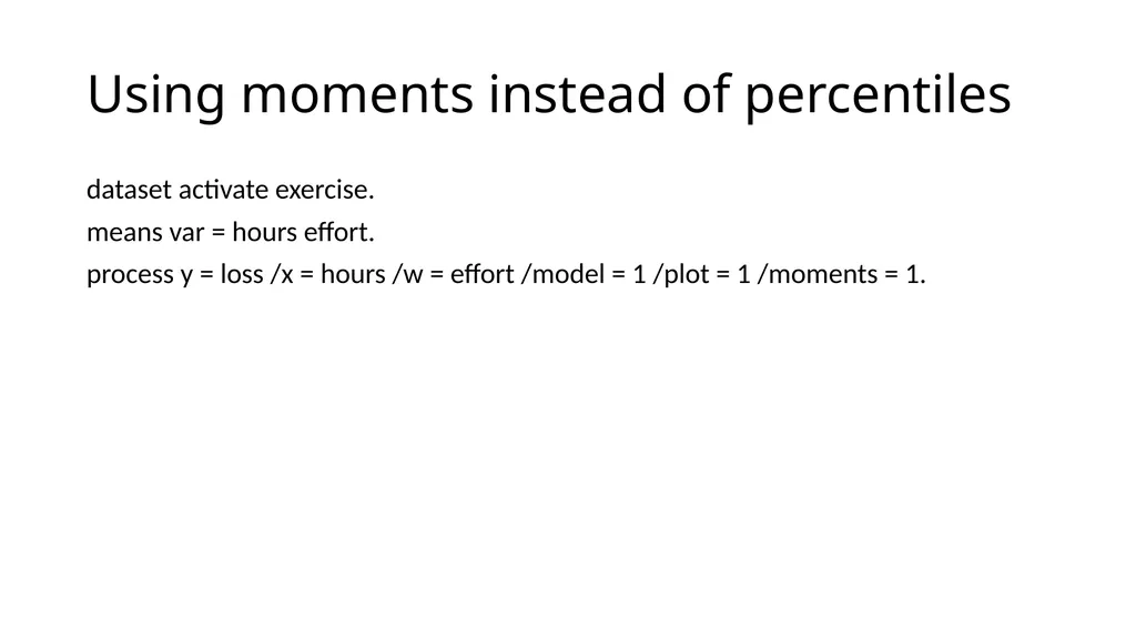
slide92. Using moments instead of percentiles dataset activate exercise.
means var = hours effort.
process y = loss /x = hours /w = effort /model = 1 /plot = 1 /moments = 1.<br>
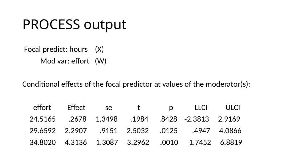
slide93. PROCESS output Focal predict: hours (X)
Mod var: effort (W)

Conditional effects of the focal predictor at values of the moderator(s):

effort Effect se t p LLCI ULCI
24.5165 .2678 1.3498 .1984 .8428 -2.3813 2.9169
29.6592 2.2907 .9151 2.5032 .0125 .4947 4.0866
34.8020 4.3136 1.3087 3.2962 .0010 1.7452 6.8819<br>
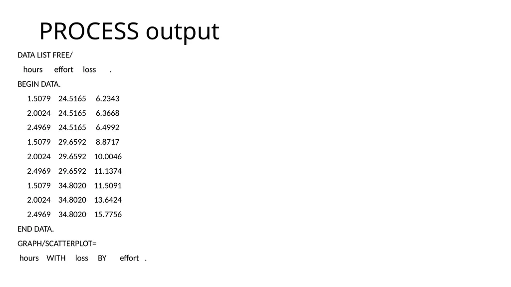
slide94. PROCESS output DATA LIST FREE/
hours effort loss .
BEGIN DATA.
1.5079 24.5165 6.2343
2.0024 24.5165 6.3668
2.4969 24.5165 6.4992
1.5079 29.6592 8.8717
2.0024 29.6592 10.0046
2.4969 29.6592 11.1374
1.5079 34.8020 11.5091
2.0024 34.8020 13.6424
2.4969 34.8020 15.7756
END DATA.
GRAPH/SCATTERPLOT=
hours WITH loss BY effort .<br>
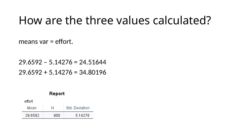
slide95. How are the three values calculated? means var = effort.

29.6592 – 5.14276 = 24.51644
29.6592 + 5.14276 = 34.80196<br>
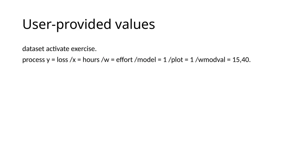
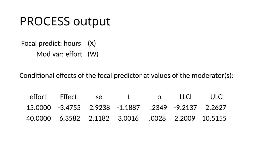
slide96. User-provided values dataset activate exercise.
process y = loss /x = hours /w = effort /model = 1 /plot = 1 /wmodval = 15,40.<br>
slide97. PROCESS output Focal predict: hours (X)
Mod var: effort (W)

Conditional effects of the focal predictor at values of the moderator(s):

effort Effect se t p LLCI ULCI
15.0000 -3.4755 2.9238 -1.1887 .2349 -9.2137 2.2627
40.0000 6.3582 2.1182 3.0016 .0028 2.2009 10.5155<br>
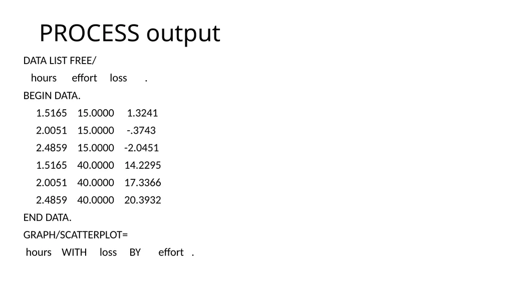
slide98. PROCESS output DATA LIST FREE/
hours effort loss .
BEGIN DATA.
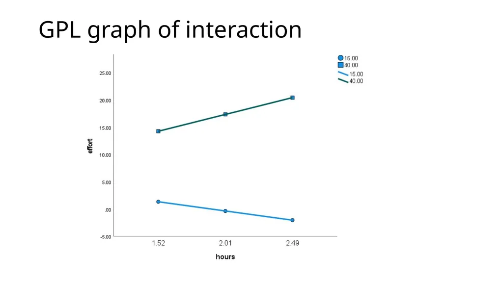
1.5165 15.0000 1.3241
2.0051 15.0000 -.3743
2.4859 15.0000 -2.0451
1.5165 40.0000 14.2295
2.0051 40.0000 17.3366
2.4859 40.0000 20.3932
END DATA.
GRAPH/SCATTERPLOT=
hours WITH loss BY effort .<br>
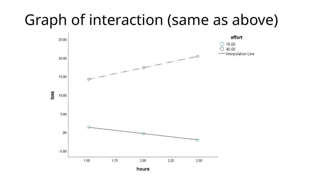
slide99. Graph of interaction (same as above)<br>
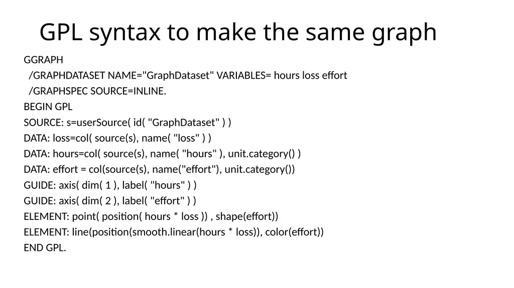
slide100. GPL syntax to make the same graph GGRAPH
/GRAPHDATASET NAME="GraphDataset" VARIABLES= hours loss effort
/GRAPHSPEC SOURCE=INLINE.
BEGIN GPL
SOURCE: s=userSource( id( "GraphDataset" ) )
DATA: loss=col( source(s), name( "loss" ) )
DATA: hours=col( source(s), name( "hours" ), unit.category() )
DATA: effort = col(source(s), name("effort"), unit.category())
GUIDE: axis( dim( 1 ), label( "hours" ) )
GUIDE: axis( dim( 2 ), label( "effort" ) )
ELEMENT: point( position( hours * loss )) , shape(effort))
ELEMENT: line(position(smooth.linear(hours * loss)), color(effort))
END GPL.<br>
slide101. GPL graph of interaction<br>
slide102. Two two-way interactionsAKA additive multiple moderation<br>
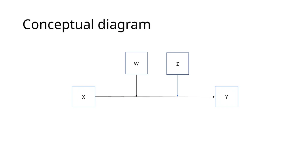
slide103. Conceptual diagram W X Y Z<br>
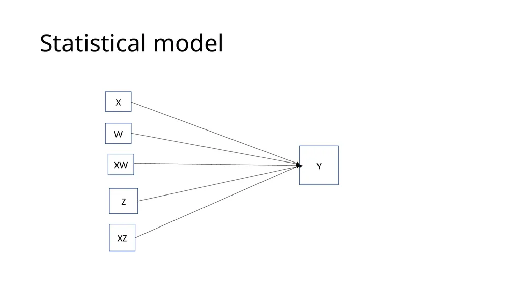
slide104. Statistical model X W XW Y Z XZ<br>
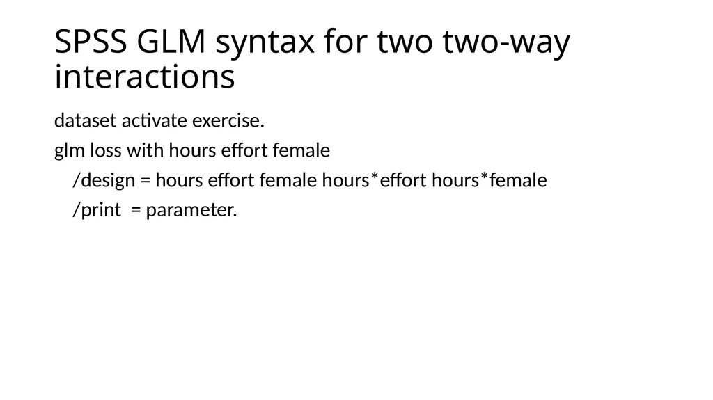
slide105. SPSS GLM syntax for two two-way interactions dataset activate exercise.
glm loss with hours effort female
/design = hours effort female hours*effort hours*female
/print = parameter.<br>
slide106. SPSS GLM output<br>
slide107. SPSS GLM output<br>
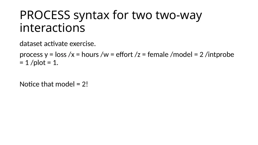
slide108. PROCESS syntax for two two-way interactions dataset activate exercise.
process y = loss /x = hours /w = effort /z = female /model = 2 /intprobe = 1 /plot = 1.

Notice that model = 2!<br>
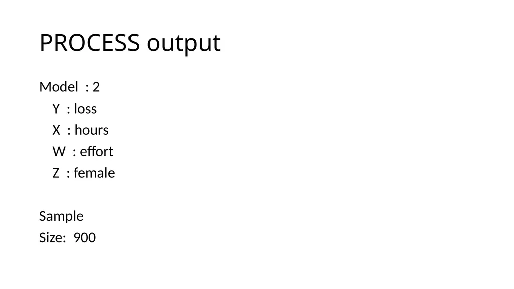
slide109. PROCESS output Model : 2
Y : loss
X : hours
W : effort
Z : female

Sample
Size: 900<br>
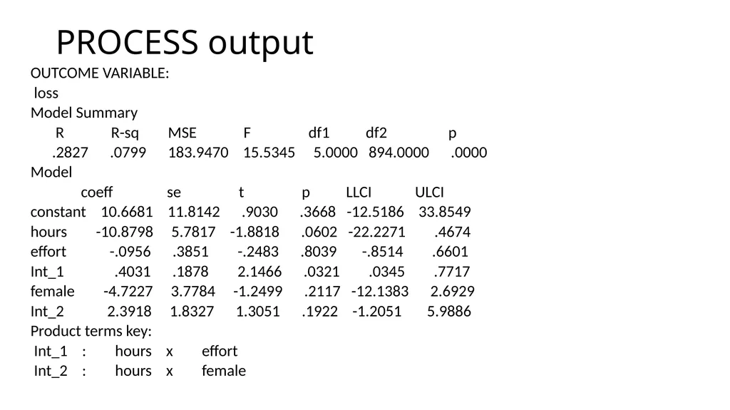
slide110. PROCESS output OUTCOME VARIABLE:
loss
Model Summary
R R-sq MSE F df1 df2 p
.2827 .0799 183.9470 15.5345 5.0000 894.0000 .0000
Model
coeff se t p LLCI ULCI
constant 10.6681 11.8142 .9030 .3668 -12.5186 33.8549
hours -10.8798 5.7817 -1.8818 .0602 -22.2271 .4674
effort -.0956 .3851 -.2483 .8039 -.8514 .6601
Int_1 .4031 .1878 2.1466 .0321 .0345 .7717
female -4.7227 3.7784 -1.2499 .2117 -12.1383 2.6929
Int_2 2.3918 1.8327 1.3051 .1922 -1.2051 5.9886
Product terms key:
Int_1 : hours x effort
Int_2 : hours x female<br>
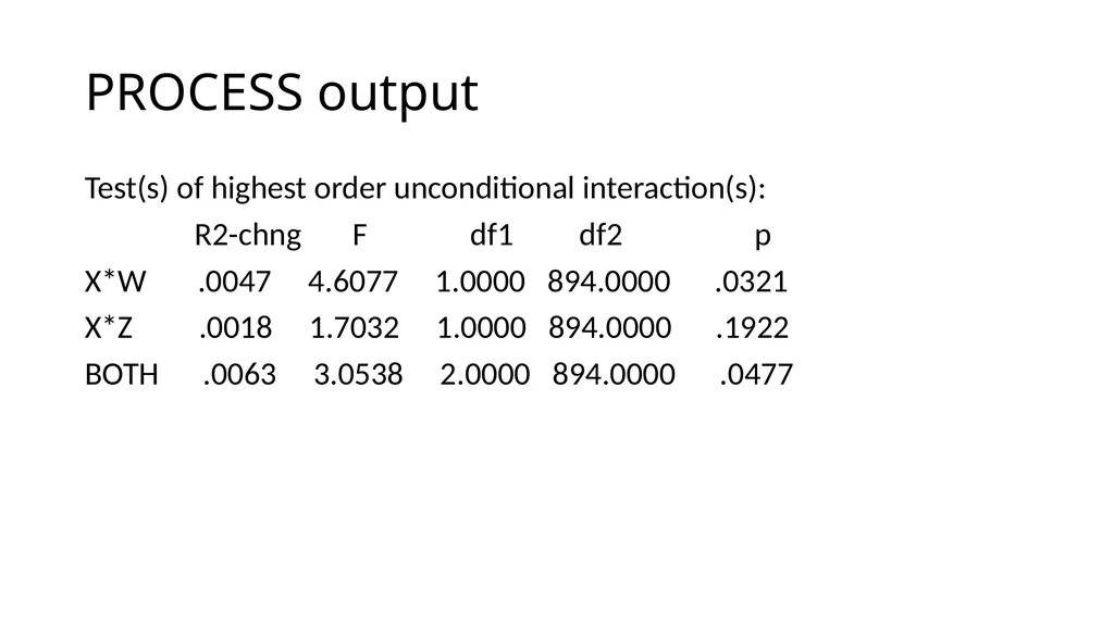
slide111. PROCESS output Test(s) of highest order unconditional interaction(s):
R2-chng F df1 df2 p
X*W .0047 4.6077 1.0000 894.0000 .0321
X*Z .0018 1.7032 1.0000 894.0000 .1922
BOTH .0063 3.0538 2.0000 894.0000 .0477<br>
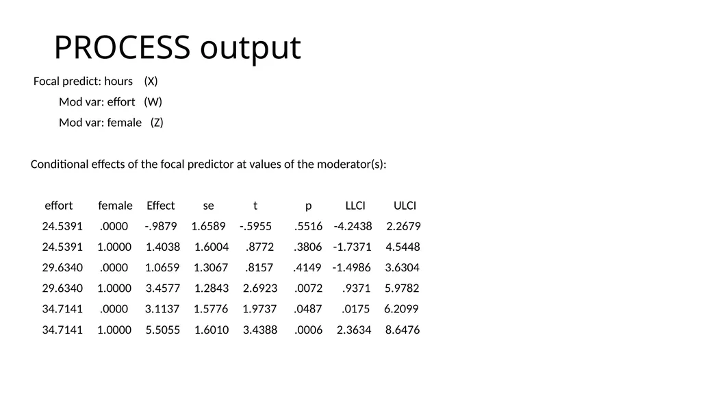
slide112. PROCESS output Focal predict: hours (X)
Mod var: effort (W)
Mod var: female (Z)

Conditional effects of the focal predictor at values of the moderator(s):

effort female Effect se t p LLCI ULCI
24.5391 .0000 -.9879 1.6589 -.5955 .5516 -4.2438 2.2679
24.5391 1.0000 1.4038 1.6004 .8772 .3806 -1.7371 4.5448
29.6340 .0000 1.0659 1.3067 .8157 .4149 -1.4986 3.6304
29.6340 1.0000 3.4577 1.2843 2.6923 .0072 .9371 5.9782
34.7141 .0000 3.1137 1.5776 1.9737 .0487 .0175 6.2099
34.7141 1.0000 5.5055 1.6010 3.4388 .0006 2.3634 8.6476<br>
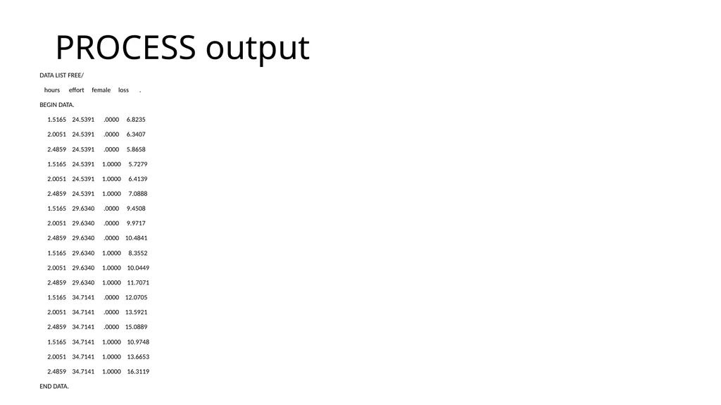
slide113. PROCESS output DATA LIST FREE/
hours effort female loss .
BEGIN DATA.
1.5165 24.5391 .0000 6.8235
2.0051 24.5391 .0000 6.3407
2.4859 24.5391 .0000 5.8658
1.5165 24.5391 1.0000 5.7279
2.0051 24.5391 1.0000 6.4139
2.4859 24.5391 1.0000 7.0888
1.5165 29.6340 .0000 9.4508
2.0051 29.6340 .0000 9.9717
2.4859 29.6340 .0000 10.4841
1.5165 29.6340 1.0000 8.3552
2.0051 29.6340 1.0000 10.0449
2.4859 29.6340 1.0000 11.7071
1.5165 34.7141 .0000 12.0705
2.0051 34.7141 .0000 13.5921
2.4859 34.7141 .0000 15.0889
1.5165 34.7141 1.0000 10.9748
2.0051 34.7141 1.0000 13.6653
2.4859 34.7141 1.0000 16.3119
END DATA.<br>
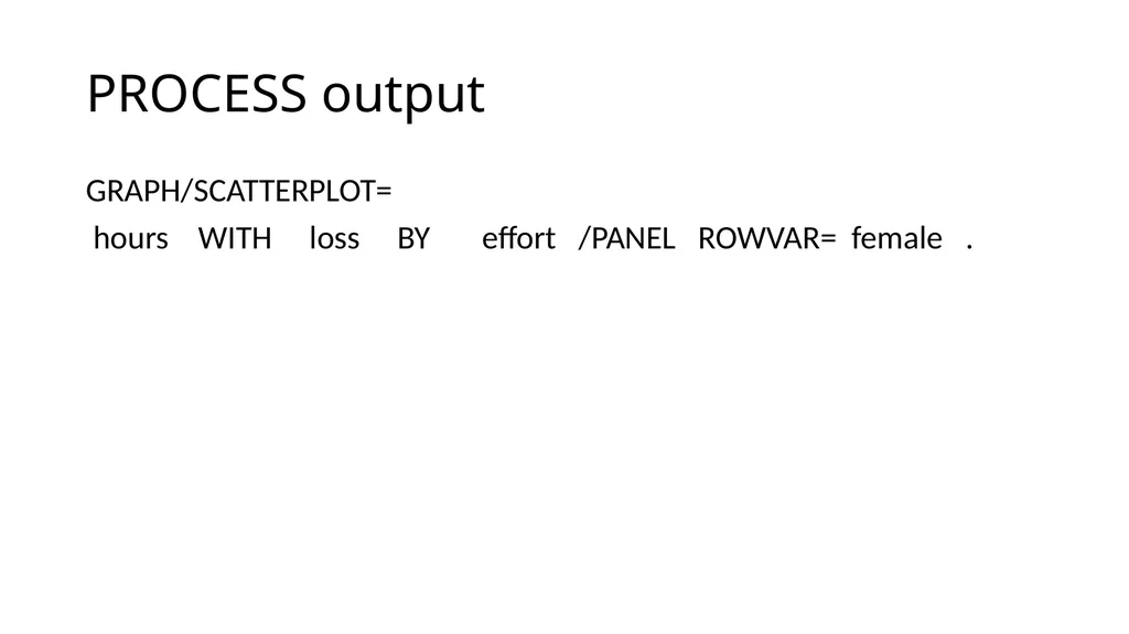
slide114. PROCESS output GRAPH/SCATTERPLOT=
hours WITH loss BY effort /PANEL ROWVAR= female .<br>
slide115. PROCESS output Level of confidence for all confidence intervals in output:
95.0000

W values in conditional tables are the 16th, 50th, and 84th percentiles.<br>
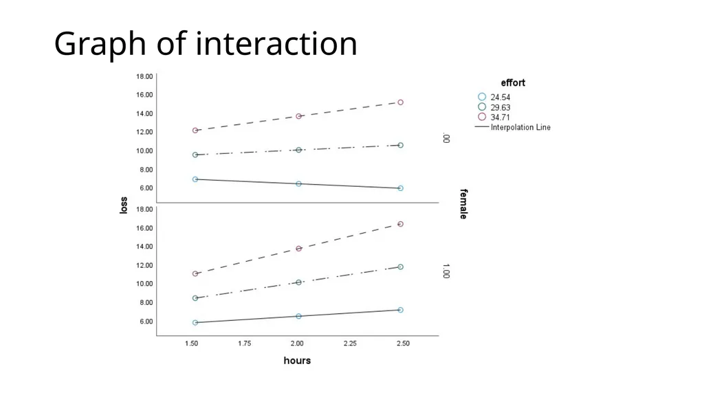
slide116. Graph of interaction<br>
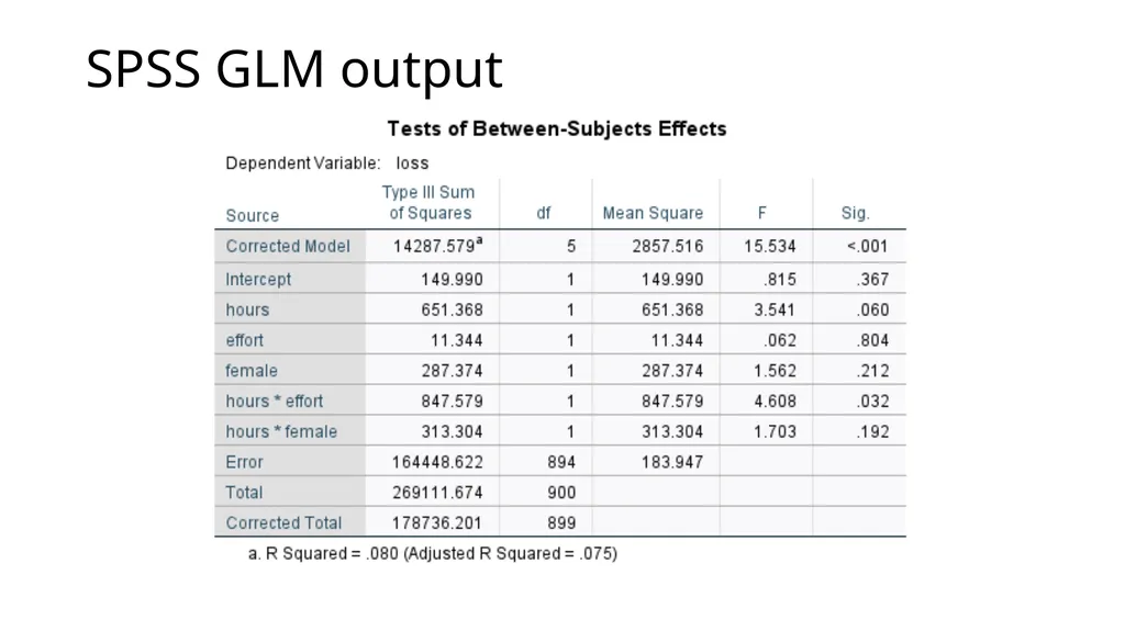
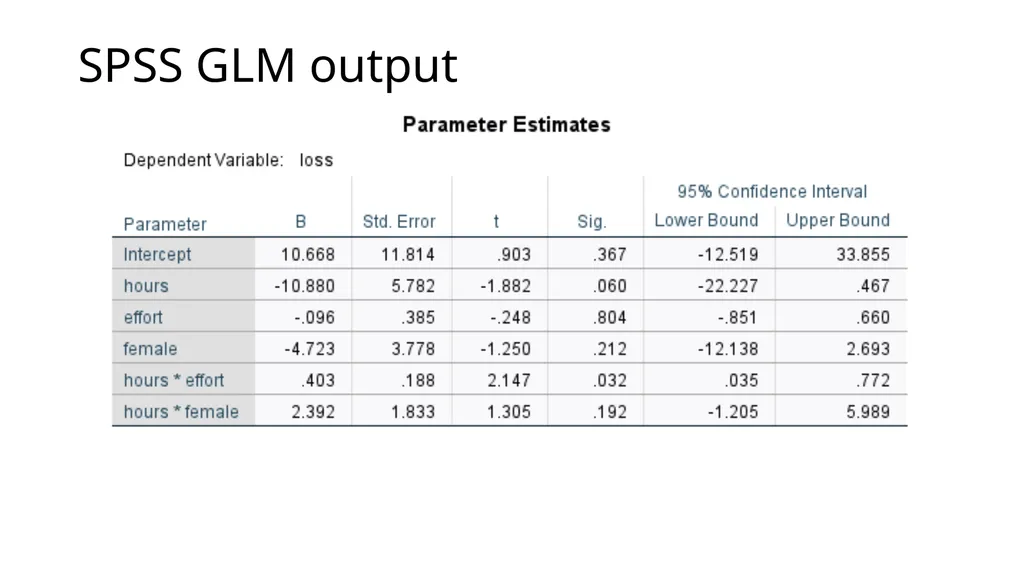
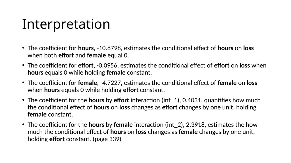
slide117. Interpretation The coefficient for hours, -10.8798, estimates the conditional effect of hours on loss when both effort and female equal 0.
The coefficient for effort, -0.0956, estimates the conditional effect of effort on loss when hours equals 0 while holding female constant.
The coefficient for female, -4.7227, estimates the conditional effect of female on loss when hours equals 0 while holding effort constant.
The coefficient for the hours by effort interaction (int_1), 0.4031, quantifies how much the conditional effect of hours on loss changes as effort changes by one unit, holding female constant.
The coefficient for the hours by female interaction (int_2), 2.3918, estimates the how much the conditional effect of hours on loss changes as female changes by one unit, holding effort constant. (page 339)<br>
slide118. Three-way interactionAKA moderated moderation<br>
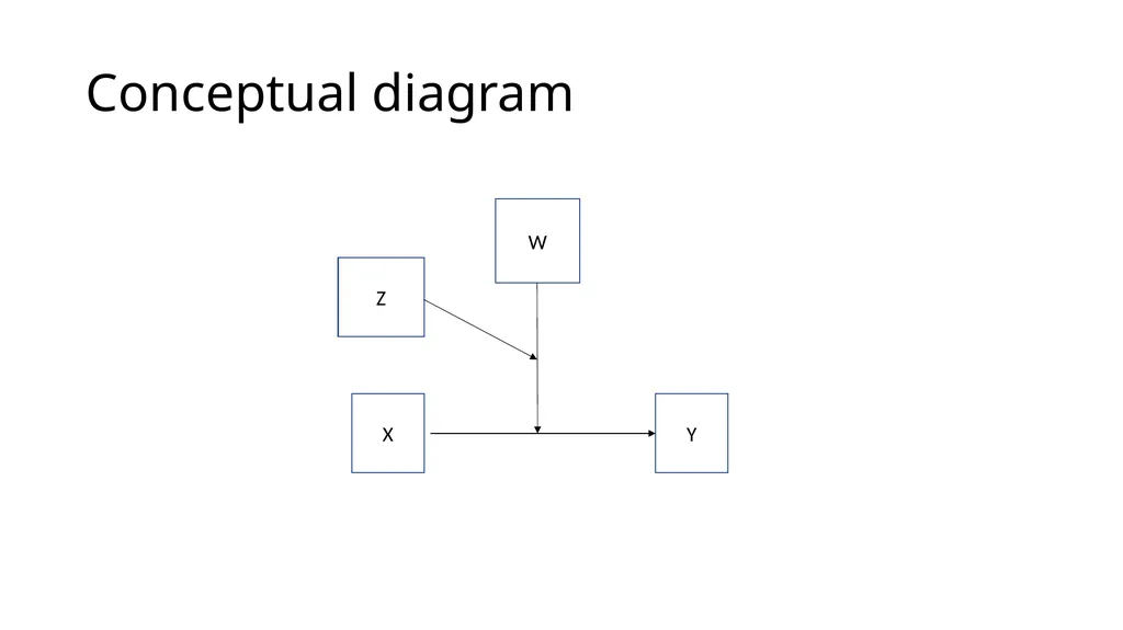
slide119. Conceptual diagram W X Y Z<br>
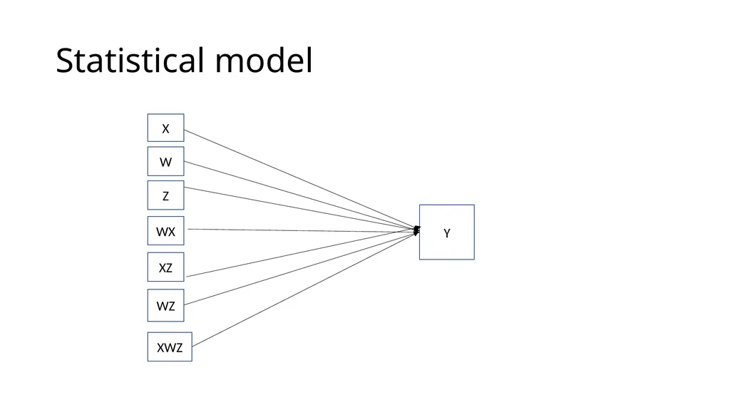
slide120. Statistical model X W Z Y WX XZ WZ XWZ<br>
slide121. Try it yourself Write the SPSS GLM syntax for a model with a three-way interaction.
Why might the output not match the PROCESS output for some coefficients?<br>
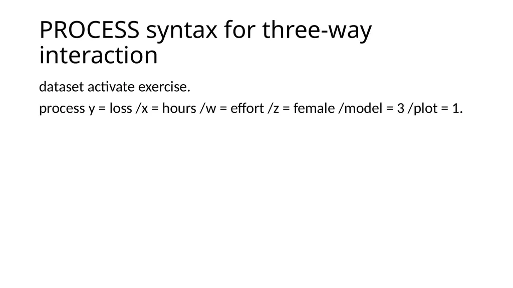
slide122. PROCESS syntax for three-way interaction dataset activate exercise.
process y = loss /x = hours /w = effort /z = female /model = 3 /plot = 1.<br>
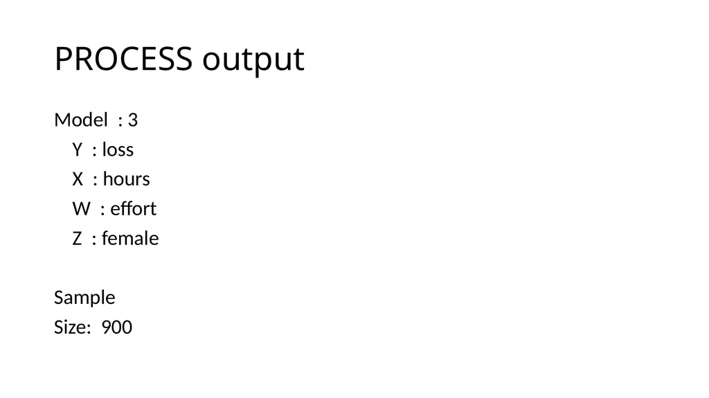
slide123. PROCESS output Model : 3
Y : loss
X : hours
W : effort
Z : female

Sample
Size: 900<br>
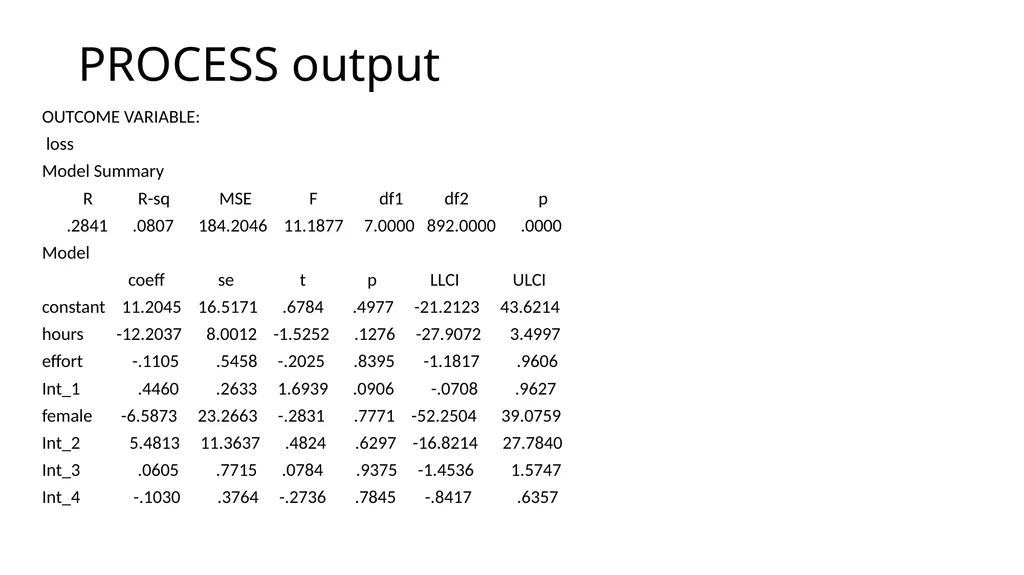
slide124. PROCESS output OUTCOME VARIABLE:
loss
Model Summary
R R-sq MSE F df1 df2 p
.2841 .0807 184.2046 11.1877 7.0000 892.0000 .0000
Model
coeff se t p LLCI ULCI
constant 11.2045 16.5171 .6784 .4977 -21.2123 43.6214
hours -12.2037 8.0012 -1.5252 .1276 -27.9072 3.4997
effort -.1105 .5458 -.2025 .8395 -1.1817 .9606
Int_1 .4460 .2633 1.6939 .0906 -.0708 .9627
female -6.5873 23.2663 -.2831 .7771 -52.2504 39.0759
Int_2 5.4813 11.3637 .4824 .6297 -16.8214 27.7840
Int_3 .0605 .7715 .0784 .9375 -1.4536 1.5747
Int_4 -.1030 .3764 -.2736 .7845 -.8417 .6357<br>
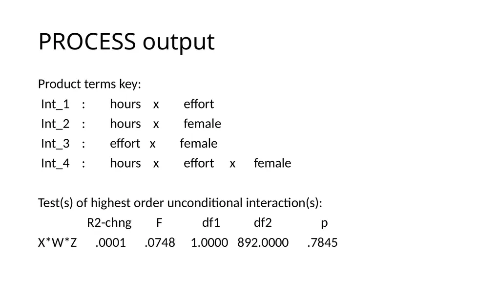
slide125. PROCESS output Product terms key:
Int_1 : hours x effort
Int_2 : hours x female
Int_3 : effort x female
Int_4 : hours x effort x female

Test(s) of highest order unconditional interaction(s):
R2-chng F df1 df2 p
X*W*Z .0001 .0748 1.0000 892.0000 .7845<br>
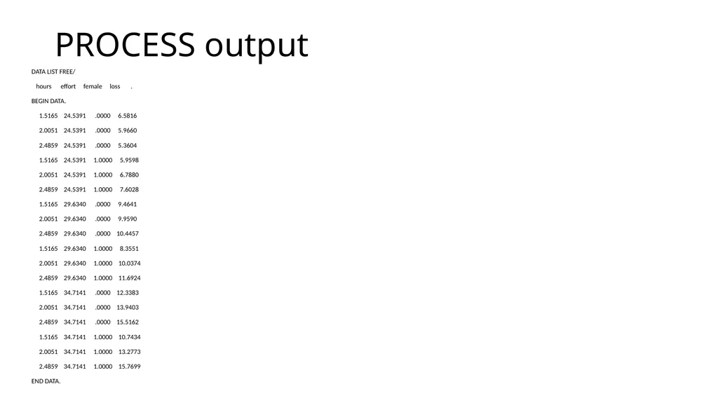
slide126. PROCESS output DATA LIST FREE/
hours effort female loss .
BEGIN DATA.
1.5165 24.5391 .0000 6.5816
2.0051 24.5391 .0000 5.9660
2.4859 24.5391 .0000 5.3604
1.5165 24.5391 1.0000 5.9598
2.0051 24.5391 1.0000 6.7880
2.4859 24.5391 1.0000 7.6028
1.5165 29.6340 .0000 9.4641
2.0051 29.6340 .0000 9.9590
2.4859 29.6340 .0000 10.4457
1.5165 29.6340 1.0000 8.3551
2.0051 29.6340 1.0000 10.0374
2.4859 29.6340 1.0000 11.6924
1.5165 34.7141 .0000 12.3383
2.0051 34.7141 .0000 13.9403
2.4859 34.7141 .0000 15.5162
1.5165 34.7141 1.0000 10.7434
2.0051 34.7141 1.0000 13.2773
2.4859 34.7141 1.0000 15.7699
END DATA.<br>
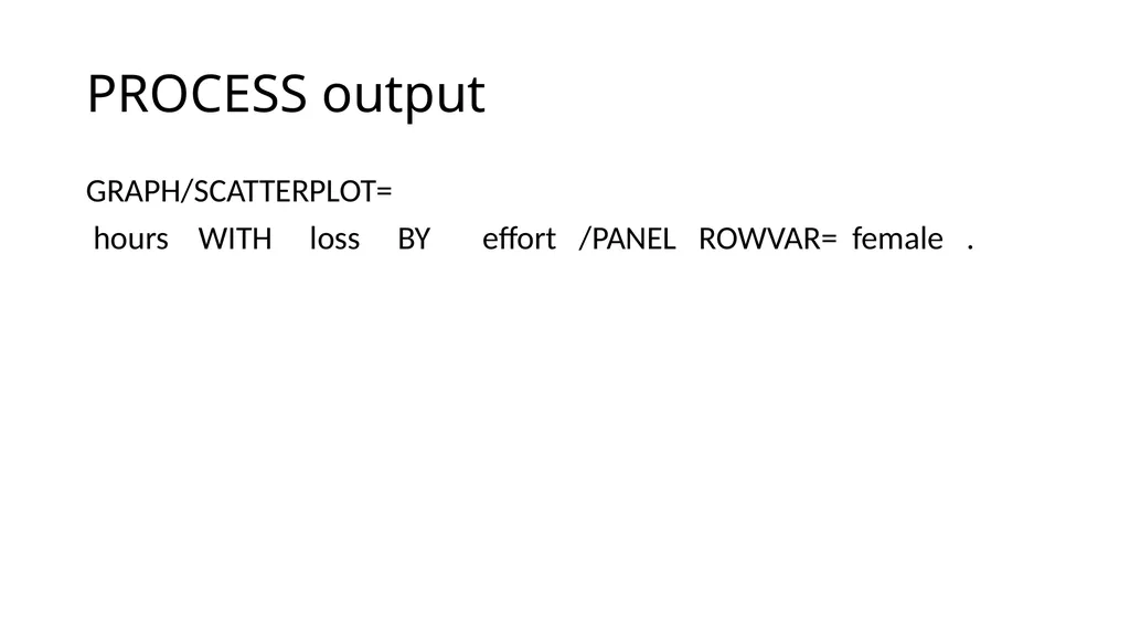
slide127. PROCESS output GRAPH/SCATTERPLOT=
hours WITH loss BY effort /PANEL ROWVAR= female .<br>
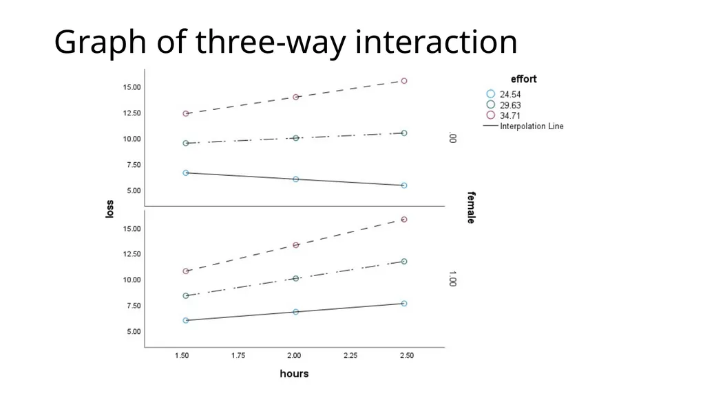
slide128. Graph of three-way interaction<br>
slide129. Interpretation “Regression coefficients for products involving X in these models quantify the rate of change of X’s effect as one moderator changes when another moderator is held fixed (additive multiple moderation) or as another moderator varies (moderated moderation).” (page 359)<br>
slide130. Try it yourself Rewrite the PROCESS syntax so that w = female and z = effort.
Run the resulting graph code.
Do you like this graph better?<br>
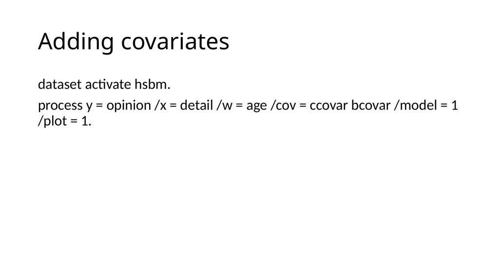
slide131. Adding covariates dataset activate hsbm.
process y = opinion /x = detail /w = age /cov = ccovar bcovar /model = 1 /plot = 1.<br>
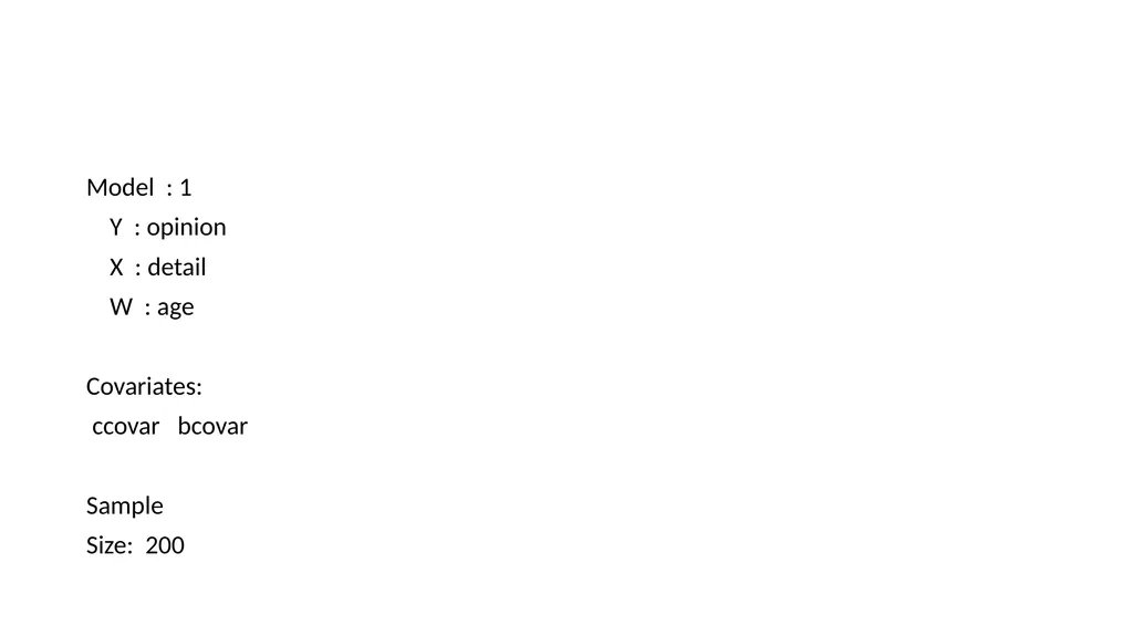
slide132. Model : 1
Y : opinion
X : detail
W : age

Covariates:
ccovar bcovar

Sample
Size: 200<br>
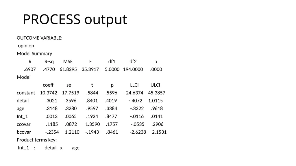
slide133. PROCESS output OUTCOME VARIABLE:
opinion
Model Summary
R R-sq MSE F df1 df2 p
.6907 .4770 61.8295 35.3917 5.0000 194.0000 .0000
Model
coeff se t p LLCI ULCI
constant 10.3742 17.7519 .5844 .5596 -24.6374 45.3857
detail .3021 .3596 .8401 .4019 -.4072 1.0115
age .3148 .3280 .9597 .3384 -.3322 .9618
Int_1 .0013 .0065 .1924 .8477 -.0116 .0141
ccovar .1185 .0872 1.3590 .1757 -.0535 .2906
bcovar -.2354 1.2110 -.1943 .8461 -2.6238 2.1531
Product terms key:
Int_1 : detail x age<br>
slide134. Heteroskedastic SEs dataset activate hsbm.
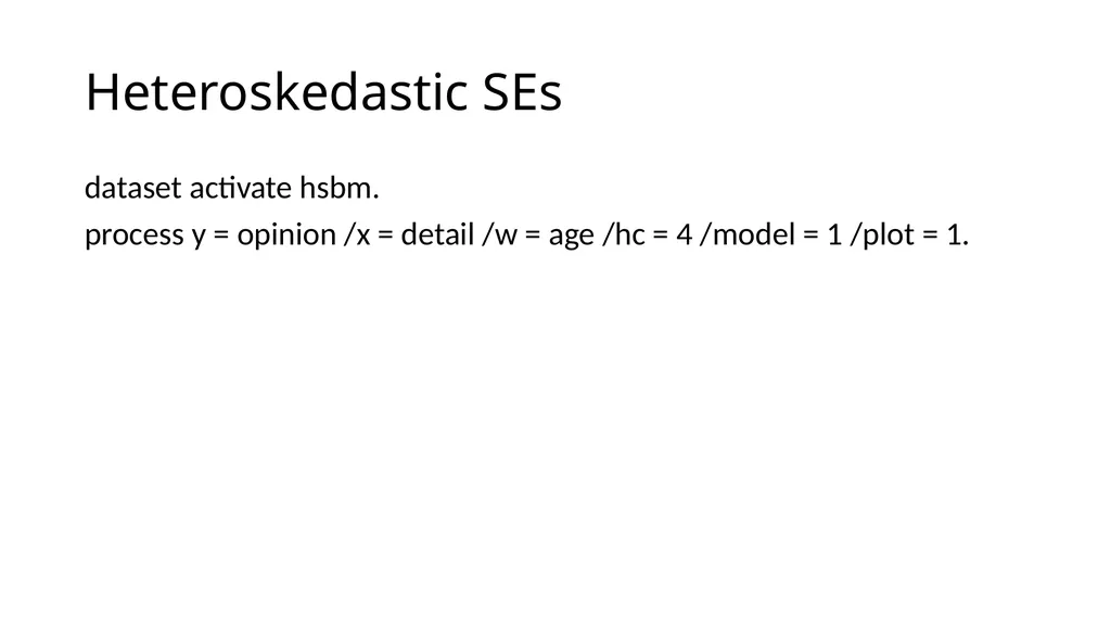
process y = opinion /x = detail /w = age /hc = 4 /model = 1 /plot = 1.<br>
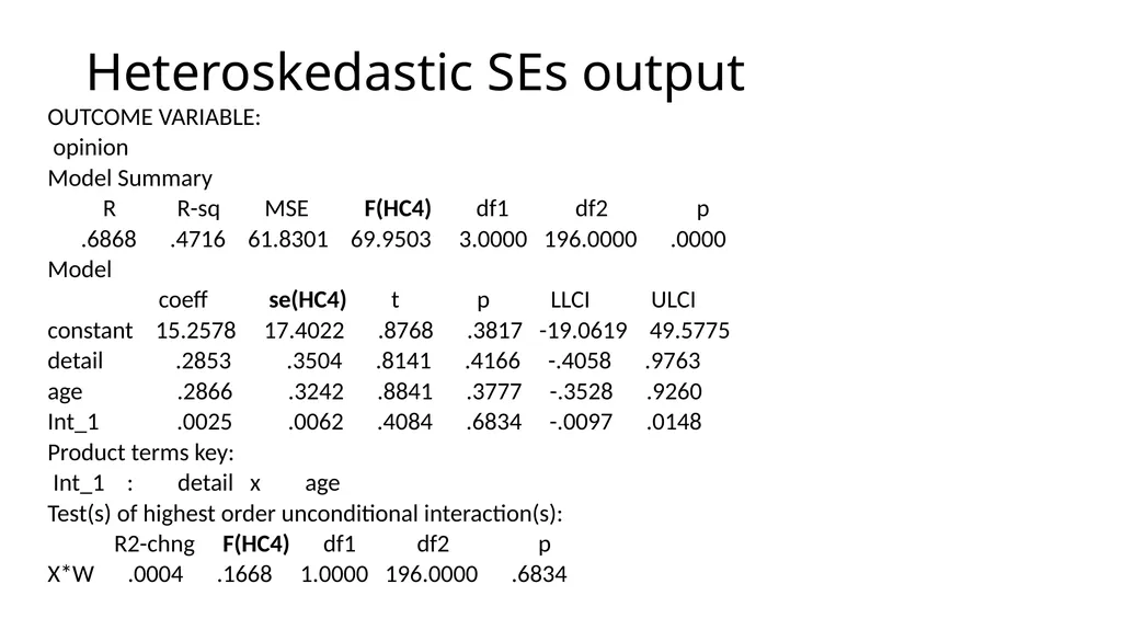
slide135. Heteroskedastic SEs output OUTCOME VARIABLE:
opinion
Model Summary
R R-sq MSE F(HC4) df1 df2 p
.6868 .4716 61.8301 69.9503 3.0000 196.0000 .0000
Model
coeff se(HC4) t p LLCI ULCI
constant 15.2578 17.4022 .8768 .3817 -19.0619 49.5775
detail .2853 .3504 .8141 .4166 -.4058 .9763
age .2866 .3242 .8841 .3777 -.3528 .9260
Int_1 .0025 .0062 .4084 .6834 -.0097 .0148
Product terms key:
Int_1 : detail x age
Test(s) of highest order unconditional interaction(s):
R2-chng F(HC4) df1 df2 p
X*W .0004 .1668 1.0000 196.0000 .6834<br>
slide136. Changing number of decimal places in output dataset activate hsbm.
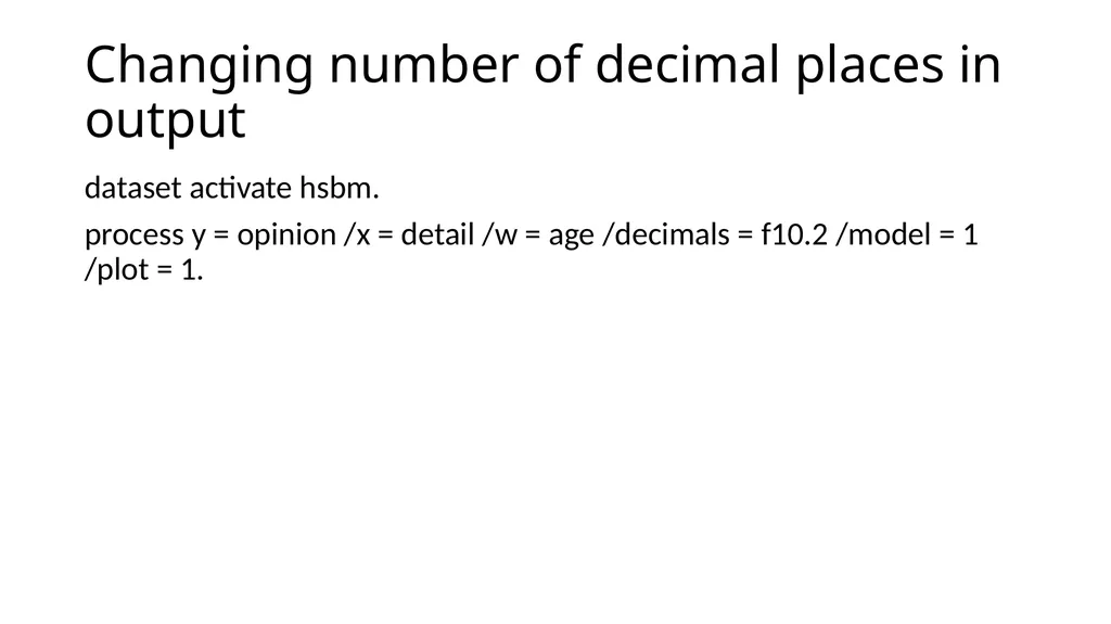
process y = opinion /x = detail /w = age /decimals = f10.2 /model = 1 /plot = 1.<br>
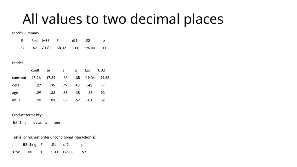
slide137. All values to two decimal places Model Summary
R R-sq MSE F df1 df2 p
.69 .47 61.83 58.32 3.00 196.00 .00

Model
coeff se t p LLCI ULCI
constant 15.26 17.39 .88 .38 -19.04 49.56
detail .29 .36 .79 .43 -.42 .99
age .29 .33 .88 .38 -.36 .93
Int_1 .00 .01 .39 .69 -.01 .02

Product terms key:
Int_1 : detail x age

Test(s) of highest order unconditional interaction(s):
R2-chng F df1 df2 p
X*W .00 .15 1.00 196.00 .69<br>
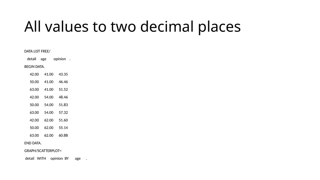
slide138. All values to two decimal places DATA LIST FREE/
detail age opinion .
BEGIN DATA.
42.00 41.00 43.35
50.00 41.00 46.46
63.00 41.00 51.52
42.00 54.00 48.46
50.00 54.00 51.83
63.00 54.00 57.32
42.00 62.00 51.60
50.00 62.00 55.14
63.00 62.00 60.88
END DATA.
GRAPH/SCATTERPLOT=
detail WITH opinion BY age .<br>
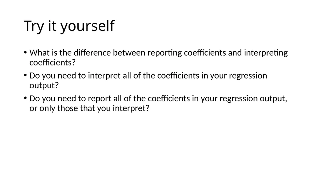
slide139. Try it yourself What is the difference between reporting coefficients and interpreting coefficients?
Do you need to interpret all of the coefficients in your regression output?
Do you need to report all of the coefficients in your regression output, or only those that you interpret?<br>
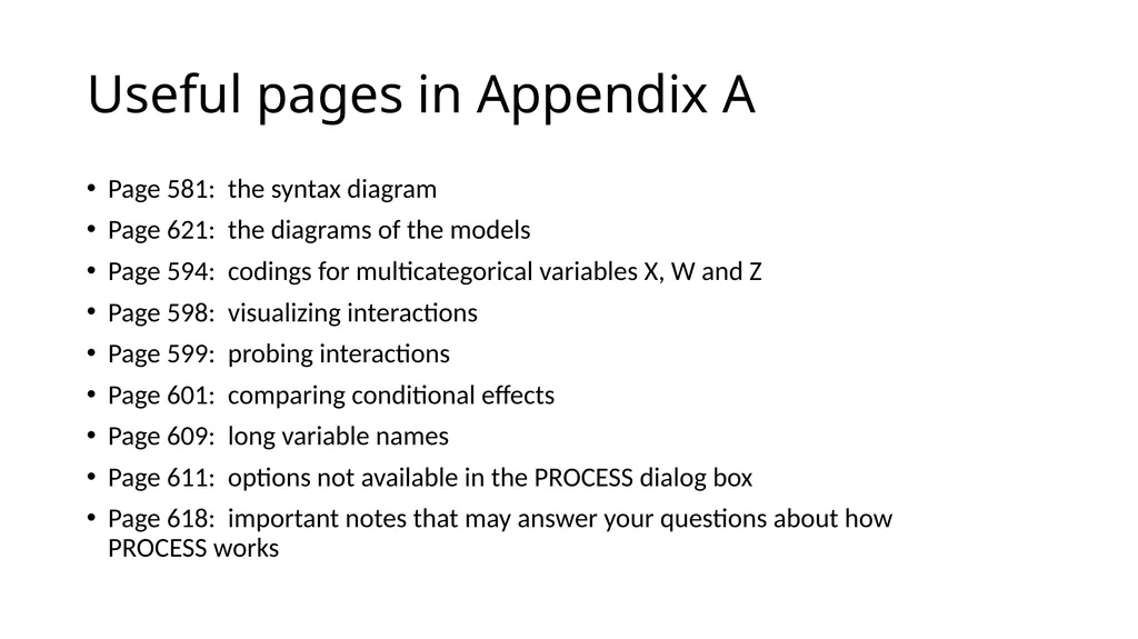
slide140. Useful pages in Appendix A Page 581: the syntax diagram
Page 621: the diagrams of the models
Page 594: codings for multicategorical variables X, W and Z
Page 598: visualizing interactions
Page 599: probing interactions
Page 601: comparing conditional effects
Page 609: long variable names
Page 611: options not available in the PROCESS dialog box
Page 618: important notes that may answer your questions about how PROCESS works<br>